Categorical Combinators for Convex Optimization and Model Predictive Control using Cvxpy
We’re gonna pump this well until someone MAKES me stop.
This particular example is something that I’ve been trying to figure out for a long time, and I am pleasantly surprised at how simple it all seems to be. The key difference with my previous abortive attempts is that I’m not attempting the heavy computational lifting myself.
We can take pointful DSLs and convert them into point-free category theory inspired interface. In this case a very excellent pointful dsl for convex optimization: cvxpy. Some similar and related posts converting dsls to categorical form
- http://www.philipzucker.com/categorical-lqr-control-with-linear-relations/
- http://www.philipzucker.com/categorical-combinators-for-graphviz-in-python/
- http://www.philipzucker.com/rough-ideas-on-categorical-combinators-for-model-checking-petri-nets-using-cvxpy/
- http://www.philipzucker.com/a-sketch-of-categorical-relation-algebra-combinators-in-z3py/
A convex optimization problem optimizes a convex objective function with constraints that define a convex set like polytopes or balls. They are polynomial time tractable and shockingly useful. We can make a category out of convex optimization problems. We consider some variables to be “input” and some to be “output”. This choice is somewhat arbitrary as is the case for many “relation” feeling things that aren’t really so rigidly oriented.
Convex programming problems do have a natural notion of composition. Check out the last chapter of Rockafeller, where he talks about the convex algebra of bifunctions. Instead of summing over the inner composition variable like in Vect $ \sum_j A_{ij}B_{jk}$, or existentializing like in Rel \(\{ (a,c) \vert \exists b. (a,b)\in A, (b,c) \in B \}\), we instead minimize over the inner composition variable $ min_y A(x,y) + B(y,z)$. These are similar operations in that they all produce bound variables.
The identity morphism is just the simple constraint that the input variables equal to output variables with an objective function of 0. This is an affine constraint, hence convex.
In general, if we ignore the objective part entirely by just setting it to zero, we’re actually working in a very computationally useful subcategory of Rel, ConvexRel, the category of relations which are convex sets. Composition corresponds to an existential operation, which is quickly solvable by convex optimization techniques. In operations research terms, these are feasibility problems rather than optimization problems. Many of the combinators do nothing to the objective.
The monoidal product just stacks variables side by side and adds the objectives and combines the constraints. They really are still independent problems. Writing things in this way opens up a possibility for parallelism. More on that some other day.
We can code this all up in python with little combinators that return the input, output, objective, constraintlist. We need to hide these in inner lambdas for appropriate fresh generation of variables.
import cvxpy as cvx
import matplotlib.pyplot as plt

class ConvexCat():
    def __init__(self,res):
        self.res = res
    def idd(n):
        def res():
            x = cvx.Variable(n)
            return x, x, 0, []
        return ConvexCat(res)
    def par(f,g):
        def res():
            x,y,o1, c1 = f()
            z,w,o2, c2 = g()
            a = cvx.hstack((x,z))
            b = cvx.hstack((y,w))
            return a , b , o1 + o2, c1 + c2 + [a == a, b == b] # sigh. Don't ask. Alright. FINE. cvxpyp needs hstacks registered to populate them with values
        return ConvexCat(res)
    def compose(g,f):
        def res():
            x,y,o1, c1 = f()
            y1,z,o2, c2 = g()
            return x , z, o1 + o2, c1 + c2 + [y == y1]
        return ConvexCat(res)
    def dup(n):
        def res():
           x = cvx.Variable(n)
           return x, cvx.vstack(x,x) , 0, []
        return ConvexCat(res)
    def __call__(self):
        return self.res()
    def run(self):
        x, y, o, c = self.res()
        prob = cvx.Problem(cvx.Minimize(o),c)
        sol = prob.solve()
        return sol, x, y, o
    def __matmul__(self,g):
        return self.compose(g)
    def __mul__(self,g):
        return self.par(g)
    def const(v):
        def res():
            x = cvx.Variable(1) # hmm. cvxpy doesn't like 0d variables. That's too bad
            return x, x, 0, [x == v]
        return ConvexCat(res)
    def converse(f):
        def res():
            a,b,o,c = f()
            return b, a, o, c
        return ConvexCat(res)
    def add(n):
        def res():
            x = cvx.Variable(n)
            return x, cvx.sum(x), 0, []
        return ConvexCat(res)
    def smul(s,n):
        def res():
            x = cvx.Variable(n)
            return x, s * x, 0, []
        return ConvexCat(res)
    def pos(n):
        def res():
            x = cvx.Variable(n, positive=True)
            return x, x, 0 , []
        return ConvexCat(res)

    # And many many more!
Now for a somewhat more concrete example: Model Predictive control of an unstable (linearized) pendulum.
Model predictive control is where you solve an optimization problem of the finite time rollout of a control system online. In other words, you take measurement of the current state, update the constraint in an optimization problem, ask the solver to solve it, and then apply the force or controls that the solver says is the best.
This gives the advantage over the LQR controller in that you can set hard inequality bounds on total force available, or positions where you wish to allow the thing to go. You don’t want your system crashing into some wall or falling over some cliff for example. These really are useful constraints in practice. You can also include possibly time dependent aspects of the dynamics of your system, possibly helping you model nonlinear dynamics of your system.
I have more posts on model predictive control here http://www.philipzucker.com/model-predictive-control-of-cartpole-in-openai-gym-using-osqp/ http://www.philipzucker.com/flappy-bird-as-a-mixed-integer-program/
Here we model the unstable point of a pendulum and ask the controller to find forces to balance the pendulum.
def controller(Cat,pend_step, pos, vel):
   acc = Cat.idd(3)
   for i in range(10):
      acc = acc @ pend_step
   init = Cat.const(pos) * Cat.const(vel) * Cat.idd(1)
   return acc @ init
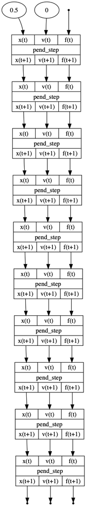
We can interpret the controller in GraphCat in order to produce a diagram of the 10 step lookahead controller. This is an advantage of the categorical style a la compiling to categories
from graphcat import *
GC = GraphCat
pend_step = GC.block("pend_step", ["x(t)", "v(t)", "f(t)"],["x(t+1)", "v(t+1)", "f(t+1)"])
pos = 0.5
vel = 0

prob = controller(GraphCat, pend_step, pos, vel)
prob.run()
We can also actually run it in model predictive control configuration in simulation.
CC = ConvexCat
idd = CC.idd

def pend_step_res():
    dt = 0.1
    x = cvx.Variable(2)
    xnext = cvx.Variable(2)
    f = cvx.Variable(1)

    pos = x[0]
    vel = x[1]
    posnext = xnext[0]
    velnext = xnext[1]
    c = []
    c += [posnext == pos + vel*dt] # position update
    c += [velnext == vel + (pos + f )* dt] # velocity update
    c += [-1 <= f, f <= 1] # force constraint
    c += [-1 <= posnext,   posnext <= 1] # safety constraint
    c += [-1 <= pos, pos <= 1]
    obj = pos**2 + posnext**2 # + 0.1 * f**2
    z = cvx.Variable(1)
    c += [z == 0]
    return cvx.hstack((x , f)) , cvx.hstack((xnext,z)), obj,  c

pend_step = ConvexCat(pend_step_res)

pos = 0.5
vel = 0
poss = []
vels = []
fs = []
dt = 0.1
'''
# we could get this to run faster if we used cvxpy params instead of recompiling the controller every time.
# some other day
p_pos = cvx.Param(1)
p_vel = cvx.Param(1)
p_pos.value = pos
p_pos.value = pos
'''
for j in range(30):

   prob = controller(ConvexCat, pend_step, pos, vel)
   _, x ,y ,_ = prob.run()
   print(x.value[2])
   #print(dir(x))
   f = x.value[2]
   #print(f)

   # actually update the state
   pos = pos + vel * dt
   vel = vel + (pos + f )* dt
   poss.append(pos)
   vels.append(vel)
   fs.append(f)
plt.plot(poss,label="pos")
plt.plot(vels, label="vel")
plt.plot(fs, label="force")
plt.legend()
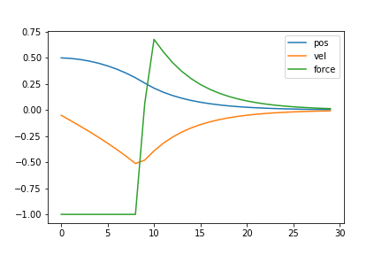 And some curves. How bout that.
Bits and Bobbles
LazySets https://github.com/JuliaReach/LazySets.jl
ADMM - It’s a “lens”. I’m pretty sure I know how to do it pointfree. Let’s do it next time.
The minimization can be bubbled out to the top is we are always minimizing. If we mix in maximization, then we can’t and we’re working on a more difficult problem. This is similar to what happens in Rel when you have relational division, which is a kind of universal quantification $ \forall$ . Mixed quantifier problems in general are very tough. These kinds of problems include games, synthesis, and robustness. More on this some other day.
Convex-Concave programming minimax https://web.stanford.edu/~boyd/papers/pdf/dccp_cdc.pdf https://web.stanford.edu/class/ee364b/lectures/cvxccv.pdf
The minimization operation can be related to the summation operation by the method of steepest descent in some cases. The method of steepest descent approximates a sum or integral by evaluating it at it’s most dominant position and expanding out from there, hence converts a linear algebra thing into an optimization problem. Examples include the connection between statistical mechanics and thermodynamics and classical mechanics and quantum mechanics.
Legendre Transformation ~ Laplace Transformation via steepest descent https://en.wikipedia.org/wiki/Convex_conjugate yada yada, all kinds of good stuff.
Intersection is easy. Join/union is harder. Does MIP help?
def meet(f,g):
   def res():
      x,y,o,c = f()
      x1,y1,o1,c1 = g()
      return x,y,o+o1, c+ c1 + [x ==  x1, y == y1]
   return res
Quantifier elimination
MIP via adjunction