Categorical LQR Control with Linear Relations
Last time, I described and built an interesting expansion of describing systems via linear functions, that of using linear relations. We remove the requirement that mappings be functional (exactly one output vector for any given input vector), which extends our descriptive capability. This is useful for describing “open” pieces of a linear system like electric circuits. This blog post is about another application: linear dynamical systems and control.
Linear relations are an excellent tool for reachability/controllability. In a control system, it is important to know where it is possible to get the system to. With linear dynamics $ x_{t+1} = Ax_{t} + B u_{t}$, an easy controllability question is “can my system reach into some subspace”. This isn’t quite the most natural question physically, but it is natural mathematically. My first impulse would be to ask “given the state starts in this little region over here, can it get to this little region over here”, but the subspace question is a bit easier to answer. It’s a little funky but it isn’t useless. It can detect if the control parameter only touches 1 of 2 independent dynamical systems for example. We can write the equations of motion as a linear relation and iterate composition on them. See Erbele for more.
There is a set of different things (and kind of more interesting things) that are under the purview of linear control theory, LQR Controllers and Kalman filters. The LQR controller and Kalman filter are roughly (exactly?) the same thing mathematically. At an abstract mathematical level, they both rely on the fact that optimization of a quadratic objective $ x^T Q x + r^T x + c$ with a linear constraints $ Ax=b$ is solvable in closed form via linear algebra. The cost of the LQR controller could be the squared distance to some goal position for example. When you optimize a function, you set the derivative to 0. This is a linear equation for quadratic objectives. It is a useful framework because it has such powerful computational teeth.
The Kalman filter does a similar thing, except for the problem of state estimation. There are measurements linear related to the state that you want to match with the prior knowledge of the linear dynamics of the system and expected errors of measurement and environment perturbations to the dynamics.
There are a couple different related species of these filters. We could consider discrete time or continuous time. We can also consider infinite horizon or finite horizon. I feel that discrete time and finite horizon are the most simple and fundamental so that is what we’ll stick with. The infinite horizon and continuous time are limiting cases.
We also can consider the dynamics to be fixed for all time steps, or varying with time. Varying with time is useful for the approximation of nonlinear systems, where there are different good nonlinear approximation (taylor series of the dynamics) depending on the current state.
There are a couple ways to solve a constrained quadratic optimization problem. In some sense, the most conceptually straightforward is just to solve for a span of the basis (the “V-Rep” of my previous post) and plug that in to the quadratic objective and optimize over your now unconstrained problem. However, it is commonplace and elegant in many respects to use the Lagrange multiplier method. You introduce a new parameter for every linear equality and add a term to the objective $ \lambda^T (A x - b)$. Hypothetically this term is 0 for the constrained solution so we haven’t changed the objective in a sense. It’s a funny slight of hand. If you optimize over x and $ \lambda$, the equality constraint comes out as your gradient conditions on $ \lambda$. Via this method, we convert a linearly constrained quadratic optimization problem into an unconstrained quadratic optimization problem with more variables.
Despite feeling very abstract, the value these Lagrangian variables take on has an interpretation. They are the “cost” or “price” of the equality they correspond to. If you moved the constraint by an amount $ Ax - b + \epsilon$, you would change the optimal cost by an amount $ \lambda \epsilon$. (Pretty sure I have that right. Units check out. See Boyd https://www.youtube.com/watch?v=FJVmflArCXc)
The Lagrange multipliers enforcing the linear dynamics are called the co-state variables. They represent the “price” that the dynamics cost, and are derivatives of the optimal value function V(s) (The best value that can be achieved from state s) that may be familiar to you from dynamic programming or reinforcement learning. See references below for more.
Let’s get down to some brass tacks. I’ve suppressed some terms for simplicity. You can also add offsets to the dynamics and costs.
A quadratic cost function with lagrange multipliers. Q is a cost matrix associated with the x state variables, R is a cost matrix for the u control variables.
\[C = \lambda_0 (x_0 - \tilde{x}_0) + \sum_t x_t^T Q x_t + u_t^T R u_t + \lambda_{t+1}^T (x_{t+1} - A x_t - B u_t )\]Equations of motion results from optimizing with respect to $ \lambda$ by design.
$ \nabla_{\lambda_{t+1}} C = x_{t+1} - A x_t - B u_t = 0$.
The initial conditions are enforced by the zeroth multiplier.
$ \nabla_{\lambda_0} C = x_i - x_{0} = 0$
Differentiation with respect to the state x has the interpretation of backwards iteration of value derivative, somewhat related to what one finds in the Bellman equation.
$ \nabla_{x_t} C = Q x_{t} + A^T \lambda_{t+1} - \lambda_{t} = 0 \Longrightarrow \lambda_{t} = A^T \lambda_{t+1} + Q x_{t}$
The final condition on value derivative is the one that makes it the most clear that the Lagrange multiplier has the interpretation of the derivative of the value function, as it sets it to that.
$ \nabla_{x_N} C = Q x_N - \lambda_{N} = 0$
Finally, differentiation with respect to the control picks the best action given knowledge of the value function at that time step.
$ \nabla_{u_t} C = R u_{t} - B^T \lambda_t = 0$
Ok. Let’s code it up using linear relations. Each of these conditions is a separate little conceptual box. We can build the optimal control step relation by combining these updates together
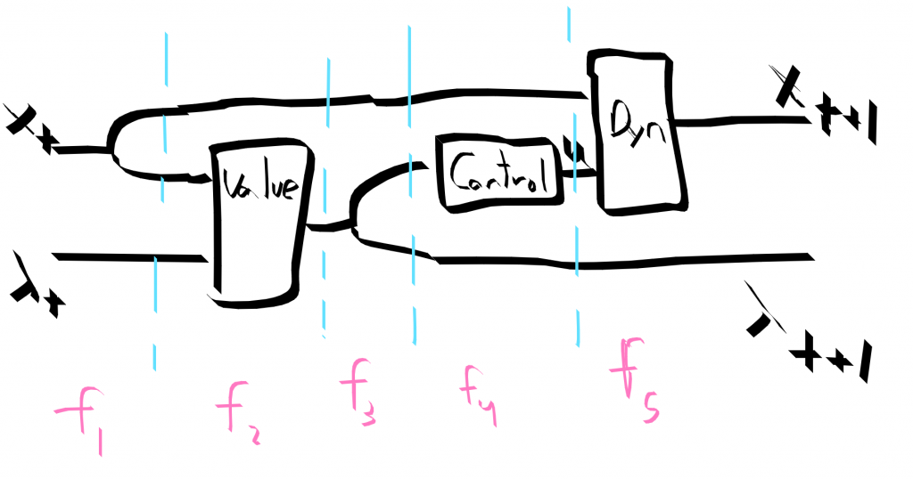 The string diagram for a single time step of control
The following is a bit sketchy. I am confident it makes sense, but I’m not confident that I have all of the signs and other details correct. I also still need to add the linear terms to the objective and offset terms to the dynamics. These details are all kind of actually important. Still, I think it’s nice to set down in preliminary blog form.
-- state of an oscillator
data SHOState = X | P deriving (Show, Enum, Bounded, Eq, Ord)
data Control = F  deriving (Show, Enum, Bounded, Eq, Ord)
-- Costate newtype wrapper
newtype Co a = Co a deriving (Show, Enum, Bounded, Eq, Ord)

type M = Matrix Double
dynamics :: forall x u. (BEnum x, BEnum u) =>  Matrix Double -> Matrix Double ->
  HLinRel (Either x u) x
dynamics a b =  HLinRel (a ||| b ||| -i )  (vzero cx) where
  cx = card @x
  cu = card @u
  i = ident cx

initial_cond :: forall x. BEnum x => Vector Double-> HLinRel Void x
initial_cond x0 =  HLinRel i x0 where
  cx = card @x
  i = ident cx

valueUpdate :: forall x l. (BEnum x, BEnum l) =>  M -> M -> HLinRel (Either x l) l
valueUpdate a q = HLinRel ((tr a) ||| q ||| i)  (vzero cl) where
  cl = card @l
  i = ident cl

optimal_u :: forall u l. (BEnum u, BEnum l) =>
     M -> M -> HLinRel u l
optimal_u r b = HLinRel (r ||| tr b) (vzero cu) where
  cu = card @u

step :: forall x u l. (BEnum x, BEnum u, BEnum l) => M -> M -> M -> M
        -> HLinRel (Either x l) (Either x l)
step a b r q =
  f5 <<< f4 <<< hassoc' <<< f3 <<< f2 <<< hassoc <<< f1 where
  f1 :: HLinRel (Either x l) (Either (Either x x) l)
  f1 = first hdup
  f2 :: HLinRel (Either x (Either x l)) (Either x l)
  f2 = second (valueUpdate a q)
  f3 ::  HLinRel (Either x l) (Either x (Either l l))
  f3 = second hdup
  f4 ::  HLinRel (Either (Either x l) l) (Either (Either x u) l)
  f4 = first (second (hconverse (optimal_u r b)))
  f5 ::  HLinRel (Either (Either x u) l) (Either x l)
  f5 = first (dynamics a b)

-- iterate (hcompose (step a b r q)) :: [HLinRel (Either x l) (Either x l)]
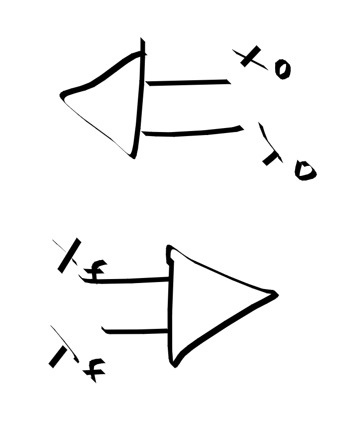 Initial conditions and final conditions. Final conditions fix the final value derivative to Qx. Initial conditions set x to some value. Should there be a leg for lambda on the initial conditions?
Bits and Bobbles
- The code in context https://github.com/philzook58/ConvexCat/blob/master/src/LinRel.hs
- Some of the juicier stuff is nonlinear control. Gotta walk before we can run though. I have some suspicions that a streaming library may be useful here, or a lens-related approach. Also ADMM.
- Reminiscent of Keldysh contour. Probably a meaningless coincidence.
- In some sense H-Rep is the analog of (a -> b -> Bool) and V-rep [(a,b)]
- Note that the equations of motion are relational rather than functional for a control systems. The control parameters $ u$ describe undetermined variables under our control.
- Loopback (trace) the value derivative for infinite horizon control.
- Can solve the Laplace equation with a Poincare Steklov operator. That should be my next post.
- There is something a touch unsatisfying even with the reduced goals of this post. Why did I have to write down the quadratic optimization problem and then hand translate it to linear relations? It’s kind of unacceptable. The quadratic optimization problem is really the most natural statement, but I haven’t figured out to make it compositional. The last chapter of Rockafellar?
References
https://arxiv.org/abs/1405.6881 Baez and Erbele - Categories in Control
https://julesh.com/2019/11/27/categorical-cybernetics-a-manifesto/
http://www.scholarpedia.org/article/Optimal_control
http://www.argmin.net/2016/05/18/mates-of-costate/ - interesting analogy to backpropagation. Lens connection?
https://courses.cs.washington.edu/courses/cse528/09sp/optimality_chapter.pdf