Linear Relation Algebra of Circuits with HMatrix

Oooh this is a fun one.

I’ve talked before about relation algebra and I think it is pretty neat. http://www.philipzucker.com/a-short-skinny-on-relations-towards-the-algebra-of-programming/. In that blog post, I used finite relations. In principle, they are simple to work with. We can perform relation algebra operations like composition, meet, and join by brute force enumeration.

Unfortunately, brute force may not always be an option. First off, the finite relations grow so enormous as to be make this infeasible. Secondly, it is not insane to talk about relations or regions with an infinite number of elements, such as some continuous blob in 2D space. In that case, we can’t even in principle enumerate all the points in the region. What are we to do? We need to develop some kind of finite parametrization of regions to manipulate. This parametrization basically can’t possibly be complete in some sense, and we may choose more or less powerful systems of description for computational reasons.

In this post, we are going to be talking about linear or affine subspaces of a continuous space. These subspaces are hyperplanes. Linear subspaces have to go through the origin, while affine spaces can have an offset from the origin.

In the previous post, I mentioned that the finite relations formed a lattice, with operations meet and join. These operations were the same as set intersection and union so the introduction of the extra terminology meet and join felt a bit unwarranted. Now the meet and join aren’t union and intersection anymore. We have chosen to not have the capability to represent the union of two vectors, instead we can only represent the smallest subspace that contains them both, which is the union closed under vector addition. For example, the join of a line and point will be the plane that goes through both.

Linear/Affine stuff is great because it is so computational. Most questions you cant to ask are answerable by readily available numerical linear algebra packages. In this case, we’ll use the Haskell package HMatrix, which is something like a numpy/scipy equivalent for Haskell. We’re going to use type-level indices to denote the sizes and partitioning of these spaces so we’ll need some helper functions.

Matrices are my patronum. They make everything good. Artwork courtesy of David

In case I miss any extensions, make typos, etc, you can find a complete compiling version here https://github.com/philzook58/ConvexCat/blob/master/src/LinRel.hs

type BEnum a = (Enum a, Bounded a) 

-- cardinality. `size` was already taken by HMatrix :(
card :: forall a. (BEnum a) => Int
card = (fromEnum (maxBound @a)) - (fromEnum (minBound @a)) + 1

In analogy with sets of tuples for defining finite relations, we partition the components of the linear spaces to be “input” and “output” indices/variables $ \begin{bmatrix} x_1 & x_2 & x_3 & … & y_1 & y_2 & y_3 & … \end{bmatrix}$. This partition is somewhat arbitrary and easily moved around, but the weakening of strict notions of input and output as compared to functions is the source of the greater descriptive power of relations.

Relations are extensions of functions, so linear relations are an extension of linear maps. A linear map has the form $ y = Ax$. A linear relation has the form $ Ax + By = 0$. An affine map has the form $ y = Ax + b$ and an affine relation has the form $ Ax + By = b$.

There are at least two useful concrete representation for subspaces.

We can write a matrix $ A$ and vector $ b$ down that corresponds to affine constraints. $ Ax = b$. The subspace described is the nullspace of $ A$ plus a solution of the equation. The rows of A are orthogonal to the space.
We can hold onto generators of subspace. $ x = A’ l+b$ where l parametrizes the subspace. In other words, the subspace is generated by / is the span of the columns of $ A’$. It is the range of $ A’$.

We’ll call these two representations the H-Rep and V-Rep, borrowing terminology from similar representations in polytopes (describing a polytope by the inequalities that define it’s faces or as the convex combination of it’s vertices). https://inf.ethz.ch/personal/fukudak/lect/pclect/notes2015/PolyComp2015.pdf These two representations are dual in many respects.

-- HLinRel holds A x = b constraint
data HLinRel a b = HLinRel (Matrix Double) (Vector Double) deriving Show

-- x = A l + b. Generator constraint. 
data VLinRel a b = VLinRel (Matrix Double) (Vector Double) deriving Show

It is useful to have both reps and interconversion routines, because different operations are easy in the two representations. Any operations defined on one can be defined on the other by sandwiching between these conversion functions. Hence, we basically only need to define operations for one of the reps (if we don’t care too much about efficiency loss which, fair warning, is out the window for today). The bulk of computation will actually be performed by these interconversion routines. The HMatrix function nullspace performs an SVD under the hood and gathers up the space with 0 singular values.

-- if A x = b then x is in the nullspace + a vector b' solves the equation
h2v :: HLinRel a b -> VLinRel a b
h2v (HLinRel a b) = VLinRel a' b' where
        b' = a <\> b -- least squares solution
        a' = nullspace a

-- if x = A l + b, then A' . x = A' A l + A' b = A' b because A' A = 0
v2h :: VLinRel a b -> HLinRel a b
v2h (VLinRel a' b') = HLinRel a b where
        b = a #> b' -- matrix multiply
        a = tr $ nullspace (tr a') -- orthogonal space to range of a.
-- tr is transpose and not trace? A little bit odd, HMatrix.

These linear relations form a category. I’m not using the Category typeclass because I need BEnum constraints hanging around. The identity relations is $ x = y$ aka $ Ix - Iy = 0$.

hid :: forall a. BEnum a => HLinRel a a
hid =  HLinRel (i ||| (- i)) (vzero s) where 
                            s = card @a
                            i = ident s

Composing relations is done by combining the constraints of the two relations and then projecting out the interior variables. Taking the conjunction of constraints is easiest in the H-Rep, where we just need to vertically stack the individual constraints. Projection easily done in the V-rep, where you just need to drop the appropriate section of the generator vectors. So we implement this operation by flipping between the two.

hcompose :: forall a b c. (BEnum a, BEnum b, BEnum c) => HLinRel b c -> HLinRel a b -> HLinRel a c
hcompose (HLinRel m b) (HLinRel m' b') = let a'' = fromBlocks [[       ma',           mb' ,    0       ],
                                                               [         0 ,    mb,        mc          ]] in
                                         let b'' = vjoin [b', b] in 
                                         let (VLinRel q p) = h2v (HLinRel a'' b'') in -- kind of a misuse
                                         let q' = (takeRows ca q)  -- drop rows belonging to @b
                                                       === 
                                                  (dropRows (ca + cb) q) in
                                         let [x,y,z] =  takesV [ca,cb,cc] p in
                                         let p'=  vjoin [x,z] in -- rebuild without rows for @b
                                         v2h (VLinRel q' p') -- reconstruct HLinRel
                                       where 
                                           ca = card @a
                                           cb = card @b 
                                           cc = card @c
                                           sb = size b -- number of constraints in first relation
                                           sb' = size b' -- number of constraints in second relation
                                           ma' = takeColumns ca m'
                                           mb' = dropColumns ca m'
                                           mb = takeColumns cb m
                                           mc = dropColumns cb m

(<<<) :: forall a b c. (BEnum a, BEnum b, BEnum c) => HLinRel b c -> HLinRel a b -> HLinRel a c
(<<<) = hcompose

We can implement the general cadre of relation operators, meet, join, converse. I feel the converse is the most relational thing of all. It makes inverting a function nearly a no-op.

hjoin :: HLinRel a b -> HLinRel a b -> HLinRel a b
hjoin v w = v2h $ vjoin' (h2v v) (h2v w)

-- hmatrix took vjoin from me :(
-- joining means combining generators and adding a new generator
-- Closed under affine combination l * x1 + (1 - l) * x2 
vjoin' :: VLinRel a b -> VLinRel a b -> VLinRel a b
vjoin' (VLinRel a b) (VLinRel a' b') = VLinRel (a ||| a' ||| (asColumn (b - b'))) b

-- no constraints, everything
-- trivially true
htop :: forall a b. (BEnum a, BEnum b) => HLinRel a b 
htop = HLinRel (vzero (1,ca + cb)) (konst 0 1) where 
                                      ca = card @a
                                      cb = card @b 

-- hbottom?

hconverse :: forall a b. (BEnum a, BEnum b) => HLinRel a b -> HLinRel b a 
hconverse (HLinRel a b) = HLinRel ( (dropColumns ca a) |||  (takeColumns ca a)) b where 
    ca = card @a
    cb = card @b  

Relational inclusion is the question of subspace inclusion. It is fairly easy to check if a VRep is in an HRep (just see plug the generators into the constraints and see if they obey them) and by using the conversion functions we can define it for arbitrary combos of H and V.

-- forall l. A' ( A l + b) == b'
-- is this numerically ok? I'm open to suggestions.
vhsub :: VLinRel a b -> HLinRel a b -> Bool
vhsub (VLinRel a b) (HLinRel a' b') = (naa' <=  1e-10 * (norm_2 a') * (norm_2 a)  ) && ((norm_2 ((a' #> b) - b')) <= 1e-10 * (norm_2 b')  ) where
          naa' = norm_2 (a' <> a)

hsub :: HLinRel a b -> HLinRel a b -> Bool
hsub h1 h2 = vhsub (h2v h1) h2

heq :: HLinRel a b -> HLinRel a b -> Bool
heq a b = (hsub a b) && (hsub b a)


instance Ord (HLinRel a b) where
  (<=) = hsub
  (>=) = flip hsub 

instance Eq (HLinRel a b) where
  (==) = heq

It is useful the use the direct sum of the spaces as a monoidal product.

hpar :: HLinRel a b -> HLinRel c d -> HLinRel (Either a c) (Either b d)
hpar (HLinRel mab v) (HLinRel mcd v') = HLinRel (fromBlocks [ [mab, 0], [0 , mcd]]) (vjoin [v, v']) where

hleft :: forall a b. (BEnum a, BEnum b) => HLinRel a (Either a b)
hleft = HLinRel ( i ||| (- i) ||| (konst 0 (ca,cb))) (konst 0 ca) where 
    ca = card @a
    cb = card @b  
    i = ident ca

hright :: forall a b. (BEnum a, BEnum b) => HLinRel b (Either a b)
hright = HLinRel ( i ||| (konst 0 (cb,ca)) ||| (- i) ) (konst 0 cb) where 
    ca = card @a
    cb = card @b  
    i = ident cb

htrans :: HLinRel a (Either b c) -> HLinRel (Either a b) c 
htrans (HLinRel m v) = HLinRel m v

hswap :: forall a b. (BEnum a, BEnum b) => HLinRel (Either a b) (Either b a)
hswap = HLinRel (fromBlocks [[ia ,0,0 ,-ia], [0, ib,-ib,0]]) (konst 0 (ca + cb)) where 
        ca = card @a
        cb = card @b  
        ia = ident ca
        ib = ident cb


hsum :: forall a. BEnum a => HLinRel (Either a a) a
hsum = HLinRel ( i ||| i ||| - i ) (konst 0 ca)  where 
        ca = card @a 
        i= ident ca

hdup :: forall a. BEnum a => HLinRel a (Either a a)
hdup = HLinRel (fromBlocks [[i, -i,0 ], [i, 0, -i]]) (konst 0 (ca + ca))  where 
        ca = card @a 
        i= ident ca

hdump :: HLinRel a Void
hdump = HLinRel 0 0

hlabsorb ::forall a. BEnum a => HLinRel (Either Void a) a
hlabsorb = HLinRel m v where (HLinRel m v) = hid @a 

A side note: Void causes some consternation. Void is the type with no elements and is the index type of a 0 dimensional space. It is the unit object of the monoidal product. Unfortunately by an accident of the standard Haskell definitions, actual Void is not a BEnum. So, I did a disgusting hack. Let us not discuss it more.

Circuits

Baez and Fong have an interesting paper where they describe building circuits using a categorical graphical calculus. We have the pieces to go about something similar. What we have here is a precise way in which circuit diagrams can be though of as string diagrams in a monoidal category of linear relations.

An idealized wire has two quantities associated with it, the current flowing through it and the voltage it is at.

-- a 2d space at every wire or current and voltage.
data IV = I | V deriving (Show, Enum, Bounded, Eq, Ord)

When we connect wires, the currents must be conserved and the voltages must be equal. hid and hcompose from above still achieve that. Composing two independent circuits in parallel is achieve by hpar.

Independent resistors in parallel.

We will want some basic tinker toys to work with.

A resistor in series has the same current at both ends and a voltage drop proportional to the current

resistor :: Double -> HLinRel IV IV
resistor r = HLinRel ( (2><4)  [ 1,0,-1,   0,
                                 r, 1, 0, -1]) (konst 0 2) 

Composing two resistors in parallel adds the resistance. (resistor r1) <<< (resistor r2) == resistor (r1 + r2))

A bridging resistor allows current to flow between the two branches

bridge :: Double -> HLinRel (Either IV IV) (Either IV IV)
bridge r = HLinRel (  (4><8) [ 1,0, 1,  0, -1, 0, -1,  0, -- current conservation
                               0, 1, 0, 0, 0, -1 , 0,  0, --voltage maintained left
                               0, 0, 0, 1, 0,  0,  0, -1, -- voltage maintained right
                               r, 1, 0,-1, -r,  0,  0, 0  ]) (konst 0 4)  

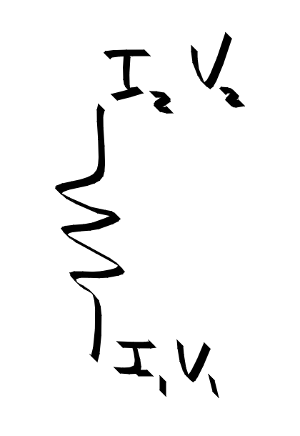
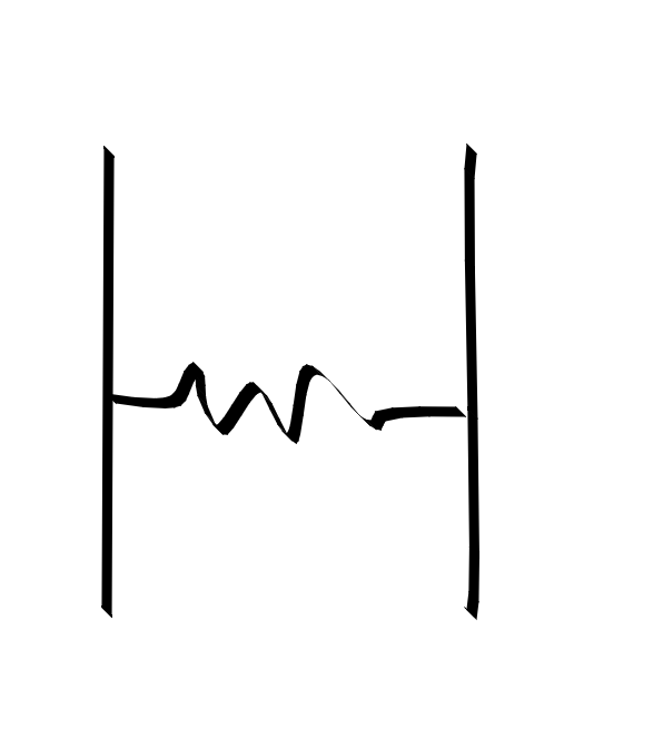A bridging resistor

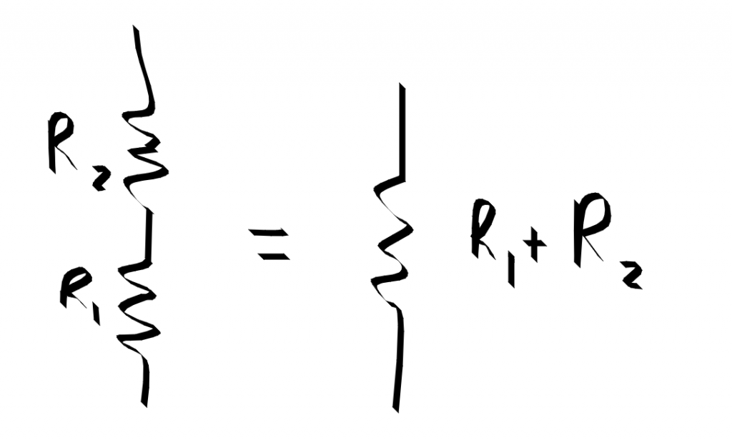
Composing two bridge circuits is putting the bridge resistors in parallel. The conductance $ G=\frac{1}{R}$ of resistors in parallel adds. hcompose (bridge r1) (bridge r2) == bridge 1 / (1/r1 + 1/r2).

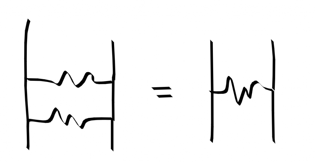parallel resistors compose

An open circuit allows no current to flow and ends a wire. open ~ resistor infinity

open :: HLinRel IV Void
open = HLinRel (fromList [[1,0]]) (konst 0 1)

At branching points, the voltage is maintained, but the current splits.

cmerge :: HLinRel (Either IV IV) IV
cmerge = HLinRel (fromList [[1, 0, 1, 0, -1, 0],
                           [0,1,0,0,0 ,-1  ],
                           [0,0,0,1, 0, -1]])  (konst 0 3)

This cmerge combinator could also be built using a short == bridge 0 , composing a branch with open, and then absorbing the Void away.

We can bend wires up or down by using a composition of cmerge and open.

cap :: HLinRel  (Either IV IV) Void
cap  = hcompose open cmerge

cup :: HLinRel Void (Either IV IV)
cup = hconverse cap

ground :: HLinRel IV Void
ground = HLinRel ( (1><2) [ 0 , 1 ]) (vzero 1) 

Voltage and current sources enforce current and voltage to be certain values

vsource :: Double -> HLinRel IV IV
vsource v = HLinRel ( (2><4) [ 1,0,-1,   0,
                               0, 1, 0, -1]) (fromList [0,v])  

isource :: Double -> HLinRel IV IV
isource i = HLinRel (fromList [ [1,0, -1,   0], -- current conservation
                                [1, 0, 0,  0]]) (fromList [0,i])  

Measurements of circuits proceed by probes.

type VProbe = ()
vprobe :: HLinRel IV VProbe
vprobe = HLinRel ( (2><3)  [1,0,0,
                            0,1,-1]) (konst 0 2)  

Inductors and capacitors could be included easily, but would require the entries of the HMatrix values to be polynomials in the frequency $ \omega$, which it does not support (but it could!). We’ll leave those off for another day.

We actually can determine that the rules suggested above are being followed by computation.

r20 :: HLinRel IV IV
r20 = resistor 20

main :: IO ()
main = do
            print (r20 == (hid <<< r20))
            print (r20 == r20 <<< hid)
            print (r20 == (hmeet r20 r20))
            print $ resistor 50 == r20 <<< (resistor 30)
            print $ (bridge 10) <<< (bridge 10) == (bridge 5)
            print $ v2h (h2v r20) == r20
            print $ r20 <= htop
            print $ hconverse (hconverse r20) == r20
            print $ (open <<< r20) == open

Bits and Bobbles

Homogenous systems are usually a bit more elegant to deal with, although a bit more unfamiliar and abstract.
Could make a pandas like interface for linear relations that uses numpy/scipy.sparse for the computation. All the swapping and associating is kind of fun to design, not so much to use. Labelled n-way relations are nice for users.
Implicit/Lazy evaluation. We should let the good solvers do the work when possible. We implemented our operations eagerly. We don’t have to. By allowing hidden variables inside our relations, we can avoid the expensive linear operations until it is useful to actually compute on them.
Relational division = quotient spaces?
DSL. One of the beauties of the pointfree/categorical approach is that you avoid the need for binding forms. This makes for a very easily manipulated DSL. The transformations feel like those of ordinary algebra and you don’t have to worry about the subtleties of index renaming or substitution under binders.
Sparse is probably really good. We have lots of identity matrices and simple rearrangements. It is very wasteful to use dense operations on these.
Schur complement https://en.wikipedia.org/wiki/Schur_complement are the name in the game for projecting out pieces of linear problems. We have some overlap.
Linear relations -> Polyhedral relations -> Convex Relations. Linear is super computable, polyhedral can blow up. Rearrange a DSL to abuse Linear programming as much as possible for queries.
Network circuits. There is an interesting subclass of circuits that is designed to be pretty composable.

https://en.wikipedia.org/wiki/Two-port_network Two port networks are a very useful subclass of electrical circuits. They model transmission lines fairly well, and easily composable for filter construction.

It is standard to describe these networks by giving a linear function between two variables and the other two variables. Depending on your choice of which variables depend on which, these are called the z-parameters, y-parameters, h-parameters, scattering parameters, abcd parameters. There are tables of formula for converting from one form to the others. The different parameters hold different use cases for composition and combining in parallel or series. From the perspective of linear relations this all seems rather silly. The necessity for so many descriptions and the confusing relationship between them comes from the unnecessary and overly rigid requirement of have a linear function-like relationship rather than just a general relation, which depending of the circuit may not even be available (there are degenerate configurations where two of the variables do not imply the values of the other two). A function relationship is always a lie (although a sometimes useful one), as there is always back-reaction of new connections.

-- voltage divider
divider :: Double -> Double -> HLinRel (Either IV IV) (Either IV IV)
divider r1 r2 = hcompose (bridge r2) (hpar (resistor r1) hid) 

The relation model also makes clearer how to build lumped models out of continuous ones. https://en.wikipedia.org/wiki/Lumped-element_model

https://en.wikipedia.org/wiki/Transmission_line https://en.wikipedia.org/wiki/Distributed-element_model

null

Because the type indices have no connection to the actual data types (they are phantom) it is a wise idea to use smart constructors that check that the sizes of the matrices makes sense.

-- smart constructors
hLinRel :: forall a b. (BEnum a, BEnum b) => Matrix Double -> Vector Double -> Maybe (HLinRel a b) 
hLinRel m v | cols m == (ca + cb) &&  (size v == rows m)  = Just (HLinRel m v)
            |  otherwise = Nothing  where 
                 ca = card @a
                 cb = card @b  

Nonlinear circuits. Grobner Bases and polynomial relations?
Quadratic optimization under linear constraints. Can’t get it to come out right yet. Clutch for Kalman filters. Nice for many formulations like least power, least action, minimum energy principles. Edit: I did more in this direction here http://www.philipzucker.com/categorical-lqr-control-with-linear-relations/
Quadratic Operators -> Convex operators. See last chapter of Rockafellar.
Duality of controllers and filters. It is well known (I think) that for ever controller algorithm there is a filter algorithm that is basically the same thing.
- LQR - Kalman
- Viterbi filter - Value function table
- particle filter - Monte Carlo control
- Extended Kalman - iLQR-ish? Use local approximation of dynamics
- unscented kalman - ?

Circuits

Bits and Bobbles

Refs