Walk on Spheres Method in Julia
##
I saw a cool tweet (and corresponding conference paper) by Keenan Crane
https://twitter.com/keenanisalive/status/1258152669727899650?s=20
http://www.cs.cmu.edu/~kmcrane/Projects/MonteCarloGeometryProcessing/index.html
I was vaguely aware that one can use a Monte Carlo method to solve the boundary value Laplace equation $ \nabla^2 \phi = 0$ , but I don’t think I had seen the walk on spheres variant of it before. I think Crane’s point is how similar all this is to stuff graphics people already do and do well. It’s a super cool paper. Check it out.
Conceptually, I think it is plausible that the Laplace equation and a monte carlo walk are related because the static diffusion equation $ \nabla^2 n = 0$ from Fick’s law ultimately comes from the brownian motion of little guys wobbling about from a microscopic perspective.
Slightly more abstractly, both linear differential equations and random walks can be describe by matrices, a finite difference matrix (for concreteness) K and a transition matrix of jump probabilities T. The differential equation is discretized to Kx=b and the stationary probability distribution is Tp=b, where b are sources and sinks at the boundary.
The mean value property of the Laplace equation allows one to speed this process up. Instead of having a ton of little walks, you can just walk out randomly sampling on the surface of big spheres. en.wikipedia.org/wiki/Walk-on-spheres_method. Alternatively you can think of it as eventually every random walk exits a sphere, and it is at a random spot on it.
So here’s the procedure. Pick a point you want the value of $ \phi$ at. Make the biggest sphere you can that stays in the domain. Pick a random point on the sphere. If that point is on the boundary, record that boundary value, otherwise iterate. Do this many many times, then the average value of the boundaries you recorded it the value of $ \phi$
This seems like a good example for Julia use. It would be somewhat difficult to code this up efficiently in python using vectorized numpy primitives. Maybe in the future we could try parallelize or do this on the GPU? Monte carlo methods like these are quite parallelizable.
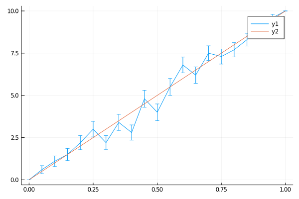
The solution of the 1-d Laplace equation is absolutely trivial. If the second derivative is 0, then . This line is found by fitting it to the two endpoint values.
So we’re gonna get a line out
using LinearAlgebra
avg = 0
phi0 = 0
phi1 = 10
x_0 = 0.75
function monte_run(x)
    while true
            l = rand(Bool) # go left?
            if (l && x <= 0.5) # finish at left edge 0
                return phi0
            elseif (!l && x >= 0.5) # finish at right edge 1
                return phi1
            else
                if x <= 0.5 # move away from 0
                    x += x
                else
                    x -= 1 - x # move away from 1
                end
            end
    end
end

monte_runs = [monte_run(x) for run_num =1:100, x=0:0.05:1 ]
import Statistics
avgs = vec(Statistics.mean( monte_runs , dims=1))
stddevs = vec(Statistics.std(monte_runs, dims=1)) ./ sqrt(size(monte_runs)[1]) # something like this right?

plot(0:0.05:1, avgs, yerror=stddevs)
plot!(0:0.05:1,  (0:0.05:1) * 10 )
And indeed we do.
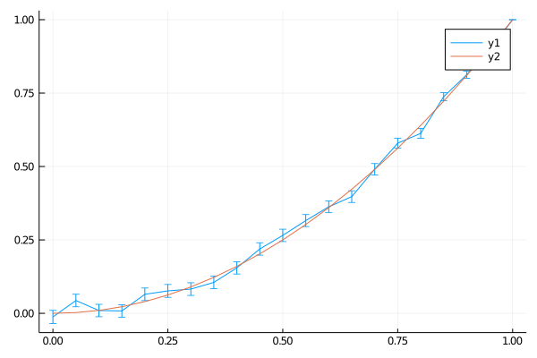
You can do a very similar thing in 2d. Here I use the boundary values on a disc corresponding to x^2 - y^2 (which is a simple exact solution of the Laplace equation).
function monte_run_2d(phi_b, x)
    while true
            r = norm(x)
            if r > 0.95 # good enough
                return phi_b(x)
            else
                dr = 1.0 - r #assuming big radius of 1
                θ = 2 * pi * rand(Float64) #
                x[1] += dr * cos(θ)
                x[2] += dr * sin(θ)
            end
    end
end


monte_run_2d( x -> x[1],  [0.0 0.0] )


monte_runs = [monte_run_2d(x -> x[1]^2 - x[2]^2 ,  [x 0.0] ) for run_num =1:1000, x=0:0.05:1 ]

import Statistics
avgs = vec(Statistics.mean( monte_runs , dims=1))
stddevs = vec(Statistics.std(monte_runs, dims=1)) ./ sqrt(size(monte_runs)[1]) # something like this right?
plot(0:0.05:1, avgs, yerror=stddevs)
plot!(0:0.05:1,  (0:0.05:1) .^2 )
There’s more notes and derivations in my notebook here https://github.com/philzook58/thoughtbooks/blob/master/monte_carlo_integrate.ipynb