Stupid Z3Py Tricks Strikes Back: Verifying a Keras Neural Network
Neural networks are all the rage these days. One mundane way of looking at neural networks is that they are a particular class of parametrized functions . What makes them useful is:
- They can be used at insane scale due to their simplicity and excellent available implementations and tooling
- There are intuitive ways to input abstract structure and symmetry expected of a problem, for example translation symmetry, or a hierarchy of small scale pattern recognition combining into large scale structures. How this all works is very peculiar.
- Inspirational analogies can be drawn from nature.
Neural networks made out of just relus (rectified linear units, relu(x) = max(0,x) ) and linear layers are particularly amenable to formal analysis. Regarding the weights as fixed (once a network has be trained), the complete neural network is a piecewise linear function. The regions where it is piecewise define are polyhedra (They are defined by the hyperplanes of the relu transitions as inequality constraints). Such functions are among those the most amenable to automated rigorous analysis.
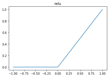 A relu
Most machine learning tasks don’t have a mathematically precise specification. What is the mathematically precise definition of a picture of a horse? We could try to come up with something (this is sort of what good old fashioned AI tried to do), but in my opinion it would be rather suspect.
Tasks that do have a precise spec are questionable areas for machine learning techniques, because how can you know that the network meets the spec? Also, one would suspect such a problem would have structure that you might be better off with a more traditional algorithmic approach.
However, there a a couple areas where one does have reasonable formal questions one might want to ask about a neural network:
- Robustness around training and validation data. Finding Adversarial examples or proving there are none.
- Games like Go. Alpha Go is a marriage of more traditional algorithmic approaches and machine learning. There is a core of traditional game tree search to it.
- Control Systems - There are many control systems which we do have a reasonable formal spec one could write, such as walking robots. These systems are so high dimensional that it is difficult to derive a good controller from the spec, and hence reinforcement learning may be a reasonable option. But we would like to confirm the controller is good and not dangerous
- Neural networks as computational accelerators. There are problems which we know how to solve, but are too slow. Neural networks can be evaluated very quickly and easily thanks to modern frameworks. It may be useful to presolve a large number of examples offline using the slow algorithm and train a neural network to give good estimates. We may be able to replace the slow thing entirely if we can verify the neural network always is good enough.
We’re going to use a neural network to fit a chebyshev polynomial. Here we’re picking a Chebyshev polynomial as our base truth because Chebyshev polynomials have some pleasant waviness to them. Why not. I like ‘em. Also polynomials are easily understood by z3 as a base spec.
This example of course is a complete toy. How often do you see 1-D input space neural networks? Not often I bet.
But it’s nice for a couple reasons:
- Because we can visualize it.
- It drives home the point about neural nets being a space of piecewise linear function approximators, and how similar training is to curve fitting.
- It’s simple enough that z3 can crush it. There is a big question if z3 or other methods can scale to realistic neural nets. Modern top of the line neural nets are insanely huge. As we’ve done it here, I highly doubt it. There are special purpose SMT solvers being built for this task. Also the slightly different technology of mixed integer programming can be used and seems very promising. So this is an area of research. See links at the bottom for more.
Generally speaking, the combination of the capabilities of sympy and z3 give us access to some very intriguing possibilities. I’m not going to investigate this in detail in this post, but I are showing how you can convert a sympy derived polynomial into a python expression using lambdify, which can then be in turn used on z3 variables.
import sympy as sy
import matplotlib.pyplot as plt
import numpy as np
x = sy.symbols('x')
cheb = sy.lambdify(x, sy.chebyshevt(4,x))
xs = np.linspace(-1,1,1000)
ys = cheb(xs)
plt.plot(xs, ys)
plt.show()
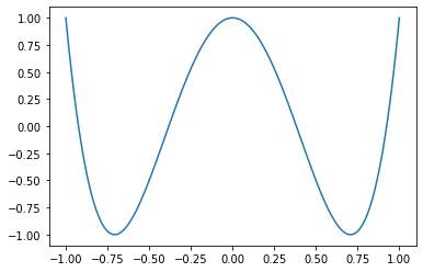 Our actual chebyshev polynomial
Here we build a very small 3 layers network using Keras. We use a least squares error and an adam optimizer. Whatever. I actually had difficulty getting nice results out for higher order chebyshev polynomials. Neural networks are so fiddly.
import tensorflow as tf
from tensorflow import keras

model = keras.Sequential([
    keras.layers.Dense(20, activation='relu', input_shape=[1]),
    keras.layers.Dense(25, activation='relu'),
    keras.layers.Dense(1)
])

optimizer = tf.keras.optimizers.Adam()

model.compile(loss='mse',
              optimizer=optimizer,
              metrics=['mae', 'mse'])

model.fit(xs, ys, epochs=100, verbose=0)
plt.plot(xs,model.predict(xs))
plt.show()
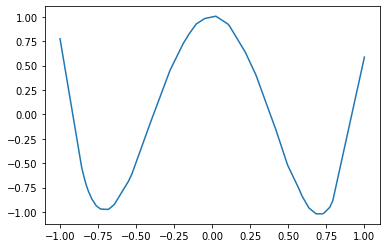 Our neural fit of the polynomial
And here we extract the weights and reinterpret them into z3. We could also have used z3 floating point capabilities rather than reals if you’re concerned about numerical issues. It was convenient to have my layers be different sizes, so that size mismatch would throw a python error. That’s how I found out the weights are transposed by default. The code at the end extracts a found countermodel and evaluates it. If you want to feel fancier, you can also use the prove function rather than an explicit Solver() instance. Saying you proved the neural network matches the polynomial to a certain tolerance feels really good. If you look at the graphs, the edges at 1 and -1 actually have pretty bad absolute error, around 0.5.
from z3 import *

w1, b1, w2, b2, w3, b3 = model.get_weights() # unpack weights from model

def Relu(x):
    return np.vectorize(lambda y: If(y >= 0 , y, RealVal(0)))(x)
def Abs(x):
    return If(x <= 0, -x, x)
def net(x):
    x1 = w1.T @ x + b1
    y1 = Relu(x1)
    x2 = w2.T @ y1 + b2
    y2 = Relu(x2)
    x3 = w3.T @ y2 + b3
    return x3

x = np.array([Real('x')])
y_true = cheb(x)
y_pred = net(x)
s = Solver()
s.add(-1 <= x[0], x[0] <= 1)
s.add(Abs( y_pred[0] - y_true[0] ) >= 0.5)
#prove(Implies( And(-1 <= x[0], x[0] <= 1),  Abs( y_pred[0] - y_true[0] ) >= 0.2))
res = s.check()
print(res)
if res == sat:
    m = s.model()
    print("Bad x value:", m[x[0]])
    x_bad = m[x[0]].numerator_as_long() / m[x[0]].denominator_as_long()
    print("Error of prediction: ", abs(model.predict(np.array([x_bad])) - cheb(x_bad)))
Links
https://github.com/sisl/NeuralVerification.jl
https://arxiv.org/abs/1711.07356 - Evaluating Robustness of Neural Networks with Mixed Integer Programming
https://github.com/vtjeng/MIPVerify.jl
https://arxiv.org/abs/1702.01135 - reluplex, SMT specifically for neural networks