Annihilating My Friend Will with a Python Fluid Simulation, Like the Cur He Is
Will, SUNDER! link to vid if not working
A color version link to vid if not working
As part of my random walk through topics, I was playing with shaders. I switched over to python because I didn’t feel like hacking out a linear solver.
There are a number of different methods for simulating fluids. I had seen Dan Piponi’s talk on youtube where he describes Jos Stam’s stable fluids and thought it made it all seem pretty straightforward. Absolutely PHENOMENAL talk. Check it out! We need to
- apply forces. I applied a gravitational force proportional to the total white of the image at that point
- project velocity to be divergence free. This makes it an incompressible fluid. We also may want to project the velocity to be zero on boundaries. I’ve done a sketchy job of that. This requires solving a Laplace equation. A sketch:
- $ v_{orig} = v_{incomp} + \nabla w$
- $ \nabla \cdot v_{incomp}=0$
- $ \nabla ^2 w = \nabla \cdot v_{orig}$. Solve for w
- $ v_{incomp}=v_{orig} - \nabla w$
- Advect using interpolation. Advect backwards in time. Use \(v(x,t+dt) \approx v(x-v(x)*dt,t)\) rather than \(v(x,t+dt) \approx v(x,t)+dv(x,t)*dt\) . This is intuitively related to the fact that backward Euler is more stable than forward Euler. Numpy had a very convenient function for this step https://docs.scipy.org/doc/scipy/reference/generated/scipy.ndimage.map_coordinates.html#scipy.ndimage.map_coordinates
Given those basic ideas, I was flying very much by the seat of my pants. I wasn’t really following any other codes. I made this to look cool. It is not a scientific calculation. I have no idea what the error is like. With a critical eye, I can definitely spot weird oscillatory artifacts. Maybe a small diffusion term would help?
When you solve for the corrections necessary to the velocity to make it incompressible $ \nabla \cdot v = 0$ , add the correction ONLY to the original field. As part of the incompressible solving step, you smooth out the original velocity field some. You probably don’t want that. By adding only the correction to the original field, you maintain the details in the original
When you discretize a domain, there are vertices, edges, and faces in your discretization. It is useful to think about upon which of these you should place your field values (velocity, pressure, electric field etc). I take it as a rule of thumb that if you do the discretization naturally, you are more likely to get a good numerical method. For example, I discretized my velocity field in two ways. A very natural way is on the edges of the graph. This is because velocity is really a stand in for material flux. The x component of the velocity belongs on the x oriented edges of the graph on the y component of velocity on the y oriented edges. If you count edges, this means that they actually in an arrays with different dimensions. There are one less edges than there are vertices.
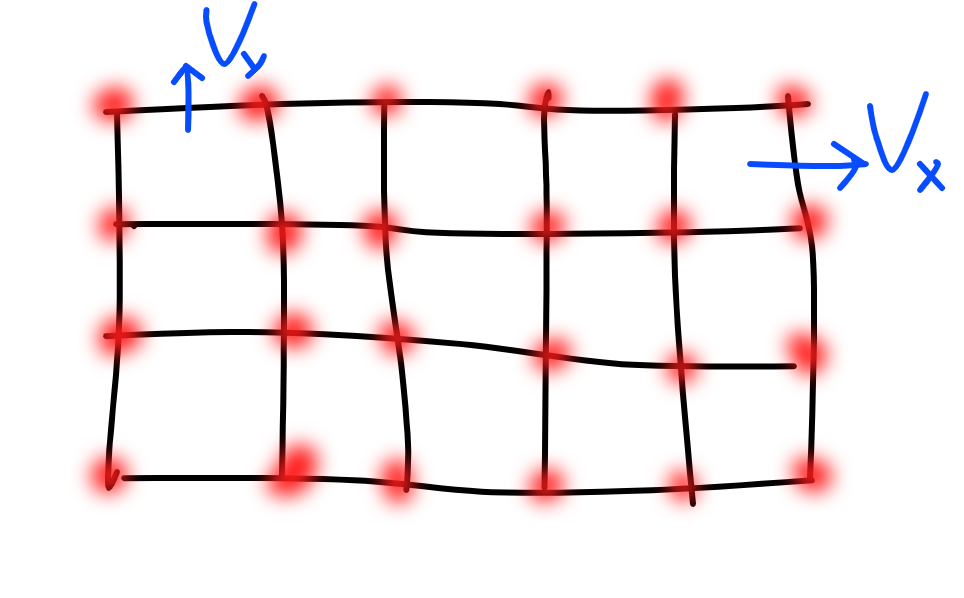 This grid is 6x4 of vertices, but the vx edges are 6x3, and the vy edges are 5x4. The boxes are a grid 5x3.
For each box, we want to constrain that the sum of velocities coming out = 0. This is the discretization of the $ \nabla \cdot v = 0$ constraint. I’m basing this on my vague recollections of discrete differential geometry and some other things I’ve see. That fields sometimes live on the edges of the discretization is very important for gauge fields, if that means anything to you. I did not try it another way, so maybe it is an unnecessary complication.
Since I needed velocities at the vertices of the grid, I do have a simple interpolation step from the vertices to the edges. So I have velocities being computed at both places. The one that is maintained between iterations lives on the vertices.
At small resolutions the code runs at real time. For the videos I made, it is probably running ~10x slower than real time. I guarantee you can make it better. Good enough for me at the moment. An FFT based Laplace solver would be fast. Could also go into GPU land? Multigrid? Me dunno.
I tried using cvxpy for the incompressibility solve, which gives a pleasant interface and great power of adding constraints, but wasn’t getting good results. i may have had a bug
This is some code just to perform the velocity projection step and plot the field. I performed the projection to 0 on the boundaries using an alternating projection method (as discussed in Piponi’s talk), which is very simple and flexible but inefficient. It probably is a lot more appropriate when you have strange changing boundaries. I could have built the K matrix system to do that too.
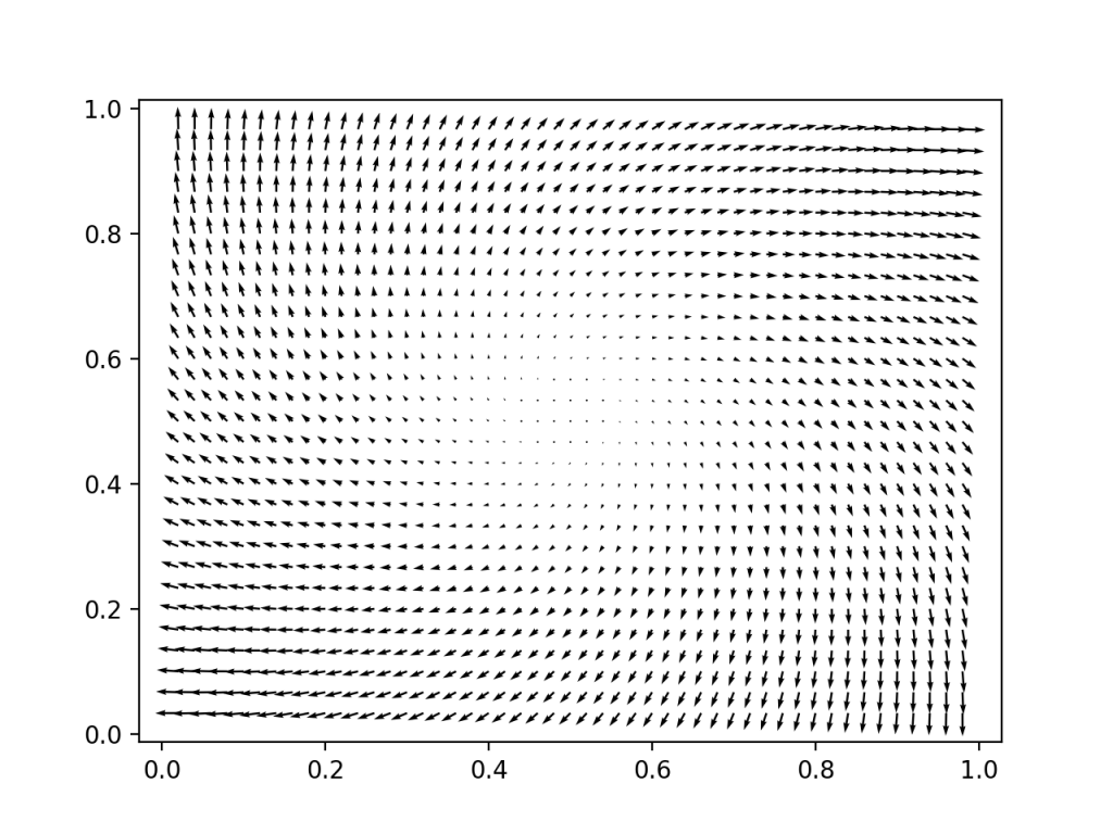 The input velocity field is spiraling outwards (not divergence free, there is a fluid source in the center)
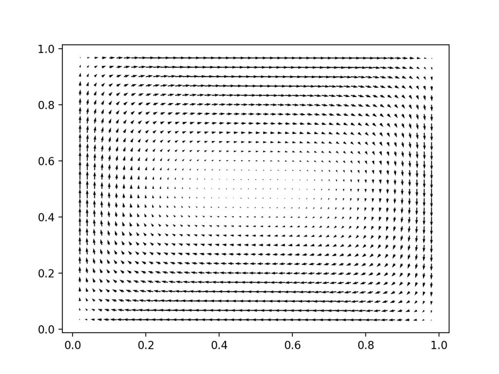 We project out the divergence free part of that velocity field, and project it such that the velocity does not point out at the boundary. Lookin good.
Presolving the laplacian matrix vastly sped up each iteration. Makes sense.
Why in gods name does sparse.kron_sum have the argument ordering it does? I had a LOT of trouble with x vs y ordering. np.meshgrid wasn’t working like I though it should. Images might have a weird convention? What a nightmare. I think it’s ok now? Looks good enough anyway.
And here is the code to make the video. I converted to image sequence to an mp4 using ffmpeg
ffmpeg -i ./%06d.jpg will.mp4
import numpy as np
import cv2
from scipy import interpolate
from scipy import ndimage
from scipy import sparse
import scipy.sparse.linalg as linalg # import spsolve

#ffmpeg -i ./%06d.jpg will.mp4

### Setup

dt = 0.01

img = cv2.imread('will.jpg')
# make image smaller to make run faster if you want
#img = cv2.pyrDown(img)
#img = cv2.pyrDown(img)

Nx = img.shape[0]
Ny = img.shape[1]


v = np.zeros((Nx,Ny,2))

x = np.linspace(0,1,Nx, endpoint=False)
y = np.linspace(0,1,Ny, endpoint=False)
X, Y = np.meshgrid(x,y, indexing='ij')

#v[:,:,0] = -Y + 0.5
#v[:,:,1] = X - 0.5


#### Build necessary derivative and interpolation matrices

def build_grad(N):
    # builds N-1 x N finite difference matrix
    data = np.array([-np.ones(N), np.ones(N-1)])
    return sparse.diags(data, np.array([0, 1]), shape= (N-1,N))

# gradient operators
gradx = sparse.kron(build_grad(Nx), sparse.identity(Ny-1))
grady = sparse.kron(sparse.identity(Nx-1), build_grad(Ny))

def build_K(N):
    # builds N-1 x N - 1   K second defivative matrix
    data = np.array([-np.ones(N-2), 2*np.ones(N-1), -np.ones(N-2)])
    diags =np.array([-1, 0, 1])
    return sparse.diags(data, diags )

# Laplacian operator . Zero dirichlet boundary conditions
# why the hell is this reversed? Sigh.
K = sparse.kronsum(build_K(Ny),build_K(Nx))
Ksolve = linalg.factorized(K)

def build_interp(N):
    data = np.array([np.ones(N)/2., np.ones(N-1)/2.])
    diags = np.array([0, 1])
    return sparse.diags(data, diags, shape= (N-1,N))
interpy = sparse.kron(sparse.identity(Nx), build_interp(Ny))
interpx = sparse.kron(build_interp(Nx), sparse.identity(Ny))


def projection_pass(vx,vy):
    # alternating projection? Not necessary. In fact stupid. but easy.
    '''
    vx[0,:] = 0
    vx[-1,:] = 0
    vy[:,0] = 0
    vy[:,-1] = 0
    '''
    vx[0,:] /= 2.
    vx[-1,:] /= 2.
    vy[:,0] /= 2.
    vy[:,-1] /= 2.

    div = gradx.dot(vx.flatten()) + grady.dot(vy.flatten()) #calculate divergence

    w = Ksolve(div.flatten())#spsolve(K, div.flatten()) #solve potential

    return gradx.T.dot(w).reshape(Nx,Ny-1), grady.T.dot(w).reshape(Nx-1,Ny)

for i in range(300):
    #while True: #
    v[:,:,0] += np.linalg.norm(img,axis=2) * dt * 0.001 # gravity force

    # interpolate onto edges
    vx = interpy.dot(v[:,:,0].flatten()).reshape(Nx,Ny-1)
    vy = interpx.dot(v[:,:,1].flatten()).reshape(Nx-1,Ny)
    # project incomperessible

    dvx, dvy = projection_pass(vx,vy)

    #interpolate change back to original grid
    v[:,:,0] -= interpy.T.dot(dvx.flatten()).reshape(Nx,Ny)
    v[:,:,1] -= interpx.T.dot(dvy.flatten()).reshape(Nx,Ny)

    #advect everything
    coords = np.stack( [(X - v[:,:,0]*dt)*Nx, (Y - v[:,:,1]*dt)*Ny], axis=0)
    print(coords.shape)
    print(v.shape)
    for j in range(3):
        img[:,:,j] = ndimage.map_coordinates(img[:,:,j], coords, order=5, mode='wrap')
    v[:,:,0] = ndimage.map_coordinates(v[:,:,0], coords, order=5, mode='wrap')
    v[:,:,1] = ndimage.map_coordinates(v[:,:,1], coords, order=5, mode='wrap')

    cv2.imshow('image',img)

    cv2.imwrite(f'will_anim3/{i:06}.jpg',img)
    k = cv2.waitKey(30) & 0xFF
    if k == ord(' '):
       break

cv2.destroyAllWindows()
Code to produce the velocity graphs above.
import cvxpy as cvx
import numpy as np
from scipy import sparse
from scipy.sparse.linalg import spsolve
import matplotlib.pyplot as plt

Nx = 50
Ny = 30
# velcitites live on the edges
vx = np.zeros((Nx,Ny-1))
vy = np.zeros((Nx-1,Ny))
x = np.linspace(0,1,Nx, endpoint=False)
y = np.linspace(0,1,Ny, endpoint=False)
X, Y = np.meshgrid(x,y, indexing='ij')
print(X[0,:])
print(X.shape)
vx[:,:] = Y[:,1:] - 1 + X[:,1:]
vy[:,:] = -X[1:,:]  + Y[1:,:]


data = np.array([-np.ones(Nx), np.ones(Nx-1)])
diags = np.array([0, 1])
grad = sparse.diags(data, diags, shape= (Nx-1,Nx))
print(grad.toarray())

gradx = sparse.kron(grad, sparse.identity(Ny-1))

data = np.array([-np.ones(Ny), np.ones(Ny-1)])
diags = np.array([0, 1])
grad = sparse.diags(data, diags, shape= (Ny-1,Ny))
print(grad.toarray())

grady = sparse.kron(sparse.identity(Nx-1), grad)
print(gradx.shape)


data = np.array([-np.ones(Nx-2), 2*np.ones(Nx-1), -np.ones(Nx-2)])
diags =np.array([-1, 0, 1])
Kx = sparse.diags(data, diags )

data = np.array([-np.ones(Ny-2), 2*np.ones(Ny-1), -np.ones(Ny-2)])
diags =np.array([-1, 0, 1])
Ky = sparse.diags(data, diags )

K = sparse.kronsum(Ky,Kx)

plt.quiver(X[1:,1:], Y[1:,1:], vx[1:,:] + vx[:-1,:], vy[:,1:] + vy[:,:-1])

for i in range(60):
    div = gradx.dot(vx.flatten()) + grady.dot(vy.flatten())
    print("div size", np.linalg.norm(div))
    div = div.reshape(Nx-1,Ny-1)

    w = spsolve(K, div.flatten())

    vx -= gradx.T.dot(w).reshape(Nx,Ny-1)
    vy -= grady.T.dot(w).reshape(Nx-1,Ny)

    # alternating projection? Not necessary. In fact stupid. but easy.
    div = gradx.dot(vx.flatten()) + grady.dot(vy.flatten())
    print("new div size", np.linalg.norm(div))
    vx[0,:] = 0
    vx[-1,:] = 0
    vy[:,0] = 0
    vy[:,-1] = 0
div = gradx.dot(vx.flatten()) + grady.dot(vy.flatten())
print("new div size", np.linalg.norm(div))

print(vx)
plt.figure()
plt.quiver(X[1:,1:], Y[1:,1:], vx[1:,:] + vx[:-1,:], vy[:,1:] + vy[:,:-1])
plt.show()
I should give a particle in cell code a try
Links
- https://github.com/PavelDoGreat/WebGL-Fluid-Simulation
- http://developer.download.nvidia.com/books/HTML/gpugems/gpugems_ch38.html
- https://www.youtube.com/watch?v=766obijdpuU
- https://pdfs.semanticscholar.org/87ad/c1196efee7d65338966f051c61bb4985421f.pdf - Jos Stam stable fluid slides
- http://taichi.graphics/links/
- https://benedikt-bitterli.me/gpu-fluid.html
Edit:
GregTJ found this post useful and made an even better simulator! Nice
()[https://www.reddit.com/r/Python/comments/fkk7aa/fluid_simulation_in_python/]