Trajectory Optimization of a Pendulum with Mixed Integer Linear Programming
There is a reasonable piecewise linear approximation for the pendulum replacing the the sinusoidal potential with two quadratic potentials (one around the top and one around the bottom). This translates to a triangle wave torque.
Cvxpy curiously has support for Mixed Integer Programming.
Cbc is probably better than GLPK MI. However, GLPK is way easier to get installed. Just brew install glpk and pip install cvxopt.
Getting cbc working was a bit of a journey. I had to actually BUILD Cylp (god forbid) and fix some problems.
Special Ordered Set constraints are useful for piecewise linear approximations. The SOS2 constraints take a set of variables and make it so that only two consecutive ones can be nonzero at a time. Solvers often have built in support for them, which can be much faster than just blasting them with general constraints. I did it by adding a binary variable for every consecutive pair. Then these binary variables suppress the continuous ones. Setting the sum of the binary variables to 1 makes only one able to be nonzero.
def SOS2(n):
	z = cvx.Variable(n-1,boolean=True)
	x = cvx.Variable(n)
	constraints = []
	constraints += [0 <= x]
	constraints += [x[0] <= z[0]]
	constraints += [x[-1] <= z[-1]]
	constraints += [x[1:-1] <= z[:-1]+z[1:]]
	constraints += [cvx.sum(z) == 1]
	constraints += [cvx.sum(x) == 1]
	return x, z, constraints
One downside is that every evaluation of these non linear functions requires a new set of integer and binary variables, which is possibly quite expensive.
For some values of total time steps and step length, the solver can go off the rails and never return.
At the moment, the solve is not fast enough for real time control with CBC (~ 2s). I wonder how much some kind of warm start might or more fiddling with heuristics, or if I had access to the built in SOS2 constraints rather than hacking it in. Also commercial solvers are usually faster. Still it is interesting.
import cvxpy as cvx
import numpy as np
import matplotlib.pyplot as plt

def SOS2(n):
	z = cvx.Variable(n-1,boolean=True)

	x = cvx.Variable(n)
	constraints = []
	constraints += [0 <= x]
	constraints += [x[0] <= z[0]]
	constraints += [x[-1] <= z[-1]]
	constraints += [x[1:-1] <= z[:-1]+z[1:]]
	constraints += [cvx.sum(z) == 1]
	constraints += [cvx.sum(x) == 1]
	return x, z, constraints


N = 20
thetas = cvx.Variable(N)
omegas = cvx.Variable(N)
torques = cvx.Variable(N)
tau = 0.3
c = [thetas[0] == +0.5, omegas[1] == 0, torques <= tau, torques >= -tau]
dt = 0.5

D = 5
thetasN = np.linspace(-np.pi,np.pi, D, endpoint=True)
zs = []
mods = []
xs = []
print(thetasN)
reward = 0
for t in range(N-1):
	c += [thetas[t+1] == thetas[t] + omegas[t]*dt]

	mod = cvx.Variable(1,integer=True)
	mods.append(mod)
	#xs.append(x)
	x, z, c1 = SOS2(D)
	c += c1
	xs.append(x)
	c += [thetas[t+1] == thetasN@x + 2*np.pi*mod]
	sin = np.sin(thetasN)@x
	reward += -np.cos(thetasN)@x
	c += [omegas[t+1] == omegas[t] - sin*dt + torques[t]*dt ]

objective = cvx.Maximize(reward)
constraints = c

prob = cvx.Problem(objective, constraints)
res = prob.solve(solver=cvx.CBC, verbose=True)

print([mod.value for mod in mods ])
print([thetasN@x.value for x in xs ])
print([x.value for x in xs ])

plt.plot(thetas.value)
plt.plot(torques.value)
plt.show()


# Other things to do: BigM.
# Disjunctive constraints.
# Implication constraints.
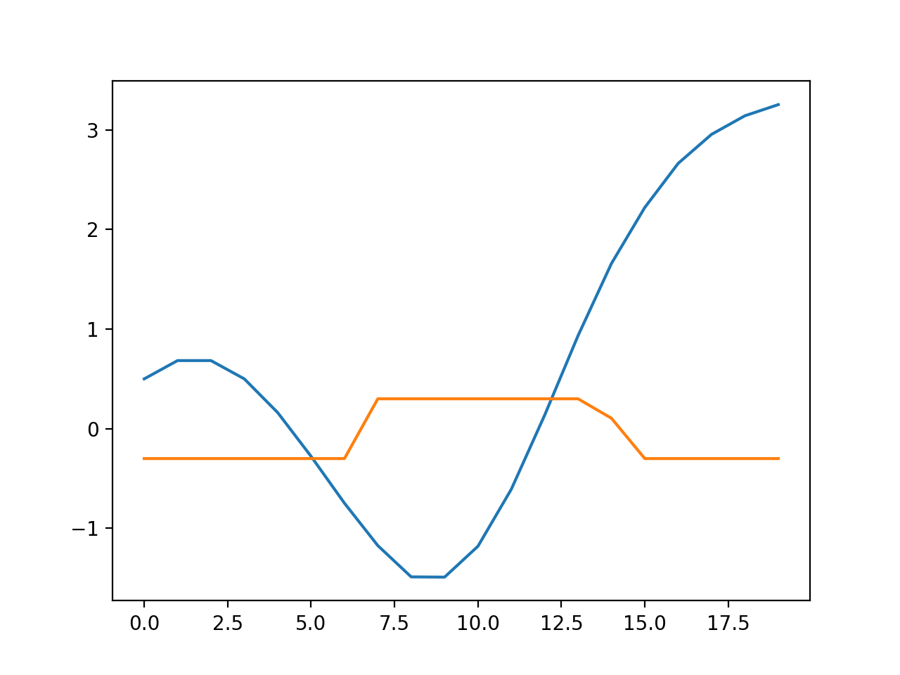 Blue is angle, orange is the applied torque. The torque is running up against the limits I placed on it.