A Touch of Topological Quantum Computation in Haskell Pt. II: Automating Drudgery
Last time we built the basic pieces we need to describe anyons in Haskell. Anyon models describe interesting physical systems where a set of particles (Tau and Id in our case) have certain splitting rules and peculiar quantum properties. The existence of anyons in a system are the core physics necessary to support topological quantum computation. In topological quantum computing, quantum gates are applied by braiding the anyons and measurements performed by fusing anyons together and seeing what particle comes out. Applying gates in this way has inherent error correcting properties.
The tree of particle production with particle labelled leaves picks a basis (think the collection $ {\hat{x}, \hat{y}, \hat{z}}$ ) for the anyon quantum vector space. An individual basis vector (think $ \hat{x}$ ) from this basis is specified by labelling the internal edges of the tree. We built a Haskell data type for a basic free vector space and functions for the basic R-moves for braiding two anyons and reassociating the tree into a new basis with F-moves. In addition, you can move around your focus within the tree by using the function lmap and rmap. The github repo with that and what follows below is here.
Pain Points
We’ve built the atomic operations we need, but they work very locally and are quite manual. You can apply many lmap and rmap to zoom in to the leaves you actually wish to braid, and you can manually perform all the F-moves necessary to bring nodes under the same parent, but it will be rather painful.
The standard paper-and-pencil graphical notation for anyons is really awesome. You get to draw little knotty squiggles to calculate. It does not feel as laborious. The human eye and hand are great at applying a sequence of reasonably optimal moves to untangle the diagram efficiently. Our eye can take the whole thing in and our hand can zip around anywhere.
To try and bridge this gap, we need to build functions that work in some reasonable way on the global anyon tree and that automate simple tasks.
A Couple Useful Functions
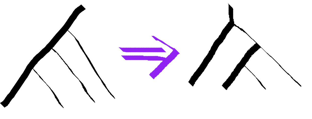
Our first useful operation is pullLeftLeaf. This operation will rearrange the tree using F-moves to get the leftmost leaf associated all the way to the root. The leftmost leaf will then have the root as a parent.
Because the tree structure is in the FibTree a b data type, we need the tuple tree type of the pulled tree. This is a slightly non-trivial type computation.
In order to do this, we’ll use a bit of typelevel programming. If this is strange and alarming stuff for you, don’t sweat it too much. I am not the most elegant user of these techniques, but I hope that alongside my prose description you can get the gist of what we’re going for.
(Sandy Maguire has a new book on typelevel programming in Haskell out. Good stuff. Support your fellow Haskeller and toss him some buckos.)
class PullLeftLeaf a b | a -> b where
  pullLeftLeaf :: FibTree c a -> Q (FibTree c b)
instance PullLeftLeaf (Tau,c) (Tau,c) where
  pullLeftLeaf = pure
instance PullLeftLeaf (Id,c) (Id,c) where
  pullLeftLeaf = pure
instance PullLeftLeaf Tau Tau where
  pullLeftLeaf = pure
instance PullLeftLeaf Id Id where
  pullLeftLeaf = pure
instance (PullLeftLeaf (a,b) (a',b'),
          r ~ (a',(b',c))) => PullLeftLeaf ((a, b),c) r where
  pullLeftLeaf t = do
           t' <- lmap pullLeftLeaf t
           fmove' t'
The resulting tree type b is an easily computable function of the starting tree type a. That is what the “functional dependency” notation | a -> b in the typeclass definition tells the compiler.
The first 4 instances are base cases. If you’re all the way at the leaf, you basically want to do nothing. pure is the function that injects the classical tree description into a quantum state vector with coefficient 1.
The meat is in the last instance. In the case that the tree type matches ((a,b),c), we recursively call PullLeftLeaf on (a,b) which returns a new result (a',b'). Because of the recursion, this a' is the leftmost leaf. We can then construct the return type by doing a single reassociation step. The notation ~ forces two types to unify. We can use this conceptually as an assignment statement at the type level. This is very useful for building intermediate names for large expressions, as assert statements to ensure the types are as expected, and also occasionally to force unification of previously unknown types. It’s an interesting operator for sure.
The recursion at the type level is completely reflected in the actual function definition. We focus on the piece (a,b) inside t by using lmap. We do a recursive call to pullLeftLeaf, and finally fmove' performs the final reassociation move. It is all rather verbose, but straightforward I hope.
You can also build a completely similar PullRightLeaf.
A Canonical Right Associated Basis
One common way of dealing with larger trees is to pick a canonical basis of fully right associated trees. The fully right associated tree is a list-like structure. Its uniformity makes it easier to work with.
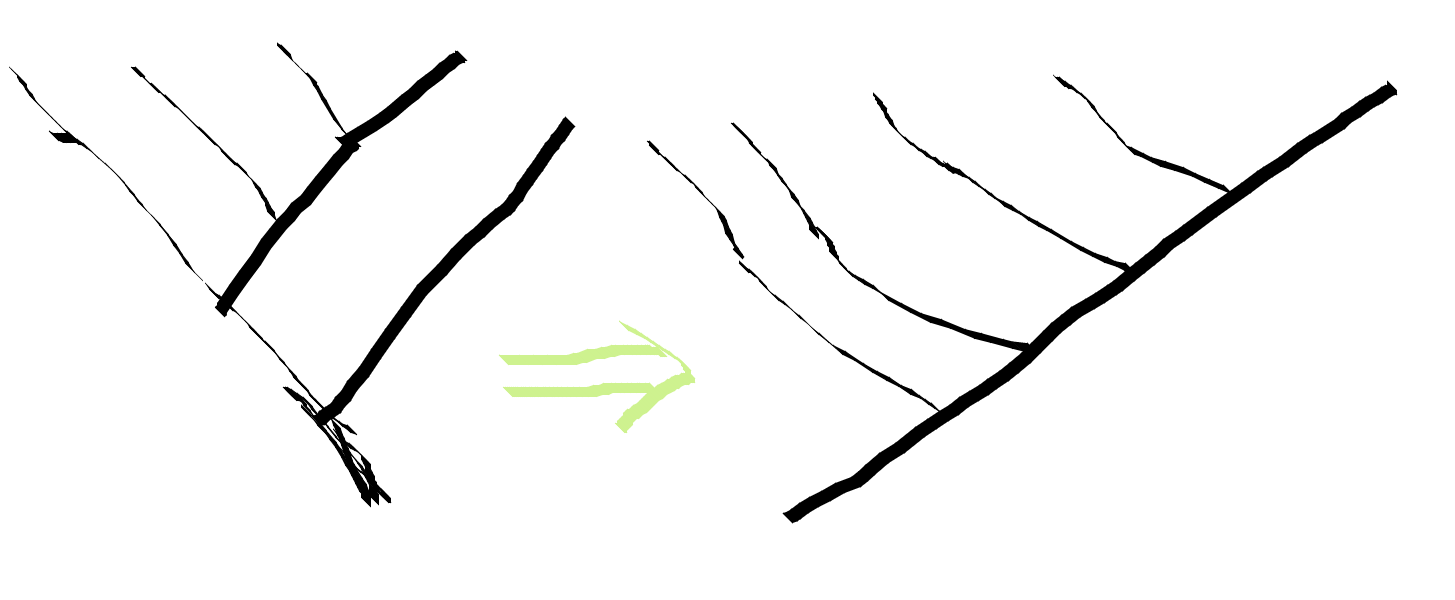
By recursively applying pullLeftLeaf, we can fully right associate any tree.
class RightAssoc a b | a -> b where
  rightAssoc :: FibTree c a -> Q (FibTree c b)
instance RightAssoc Tau Tau where
  rightAssoc = pure
instance RightAssoc Id Id where
  rightAssoc = pure
instance (PullLeftLeaf (a,b) (a',b'),
          RightAssoc b' b'',
          r ~ (a', b'')) => RightAssoc (a,b) r where
  rightAssoc t = do
           t' <- pullLeftLeaf t
           rmap rightAssoc t'
This looks quite similar to the implementation of pullLeftLeaf. It doesn’t actually have much logic to it. We apply pullLeftLeaf, then we recursively apply rightAssoc in the right branch of the tree.
B-Moves: Braiding in the Right Associated Basis
Now we have the means to convert any structure to it’s right associated canonical basis. In this basis, one can apply braiding to neighboring anyons using B-moves, which can be derived from the braiding R-moves and F-moves.
The B-move applies one F-move so that the two neighboring leaves share a parent, uses the regular braiding R-move, then applies the inverse F-move to return back to the canonical basis. Similarly, bmove' is the same thing except applies the under braiding braid' rather that the over braiding braid.
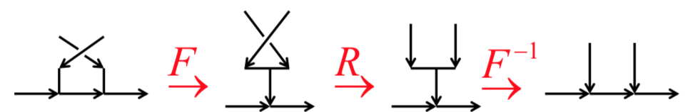
(Image Source : Preskill’s notes)
bmove :: forall b c d a. FibTree a (b,(c,d)) -> Q (FibTree a (c,(b,d)))
bmove t = do
           t'  :: FibTree a ((b,c),d) <- fmove t
           t'' :: FibTree a ((c,b),d) <-  lmap braid t'
           fmove' t''
bmove' :: forall b c d a. FibTree a (b,(c,d)) -> Q (FibTree a (c,(b,d)))
bmove' = fmove' <=< (lmap braid') <=< fmove -- point-free style for funzies. equivalent to the above except for braid'
Indexing to Leaves
We also may desire just specifying the integer index of where we wish to perform a braid. This can be achieved with another typeclass for iterated rmaping. When the tree is in canonical form, this will enable us to braid two neighboring leaves by an integer index. This index has to be a typelevel number because the output type depends on it.
In fact there is quite a bit of type computation. Given a total tree type s and an index n this function will zoom into the subpart a of the tree at which we want to apply our function. The subpart a is replaced by b, and then the tree is reconstructed into t. t is s with the subpart a mapped into b. I have intentionally made this reminiscent of the type variables of the lens type Lens s t a b .
rmapN :: forall n gte s t a b e. (RMapN n gte s t a b, gte ~ (CmpNat n 0)) => (forall r. FibTree r a -> Q (FibTree r b)) -> (FibTree e s) -> Q (FibTree e t)
rmapN f t = rmapN' @n @gte f t

class RMapN n gte s t a b | n gte s b -> a t where
    rmapN' :: (forall r. FibTree r a -> Q (FibTree r b)) -> (FibTree e s) -> Q (FibTree e t)

instance (a ~ s, b ~ t) => RMapN 0 'EQ s t a b where
    rmapN' f t = f t
instance (RMapN (n-1) gte r r' a b,
               gte ~ (CmpNat (n-1) 0),
               t ~ (l,r')) => RMapN n 'GT (l,r) t a b where
    rmapN' f t = rmap (rmapN @(n-1) f) t
This looks much noisier that it has to because we need to work around some of the unfortunate realities of using the typeclass system to compute types. We can’t just match on the number n in order to pick which instance to use because the patterns 0 and n are overlapping. The pattern n can match the number 0 if n ~ 0. The pattern matching in the type instance is not quite the same as the regular Haskell pattern matching we use to define functions. The order of the definitions does not matter, so you can’t have default cases. The patterns you use cannot be unifiable. In order to fix this, we make the condition if n is greater than 0 an explicit type variable gte. Now the different cases cannot unify. It is a very common trick to need a variable representing some branching condition.
For later convenience, we define rmapN which let’s us not need to supply the necessary comparison type gte.
Parentifying Leaves Lazily
While it is convenient to describe anyon computations in a canonical basis, it can be quite inefficient. Converting an arbitrary anyon tree into the standard basis will often result in a dense vector. A natural thing to do for the sake of economy is only do reassociation on demand.
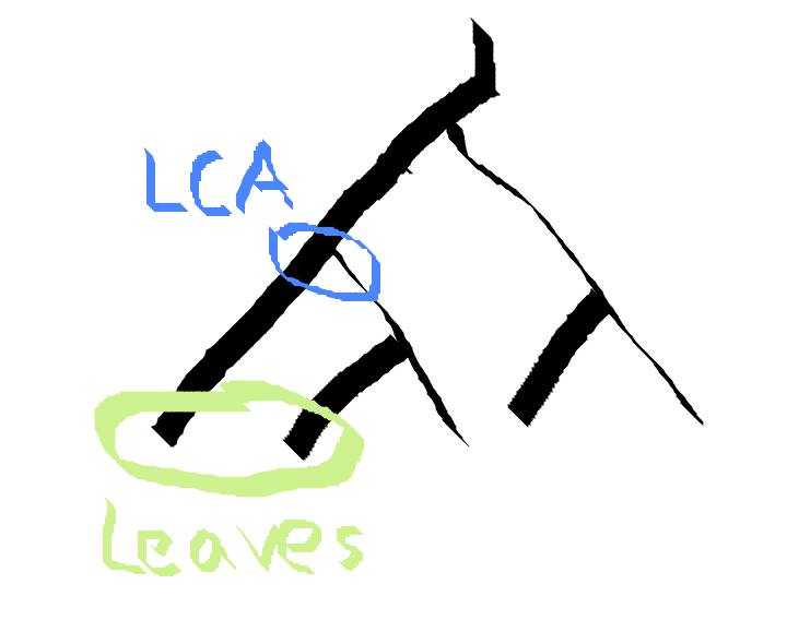
The algorithm for braiding two neighboring leaves is pretty straightforward. We need to reassociate these leaves so that they have the same parent. First we need the ability to map into the least common ancestor of the two leaves. To reassociate these two leaves to have a common parent we pullrightLeaf the left subtree and then pullLeftLeaf the left subtree. Finally, there is a bit extra bit of shuffling to actually get them to be neighbors.
As a first piece, we need a type level function to count the number of leaves in a tree. In this case, I am inclined to use type families rather than multi parameter typeclasses as before, since I don’t need value level stuff coming along for the ride.
type family Count a where
  Count Tau = 1
  Count Id = 1
  Count (a,b) = (Count a) + (Count b)

type family LeftCount a where
  LeftCount (a,b) = Count a
Next, we make a typeclass for mapping into the least common ancestor position.
lcamap ::  forall n s t a b e gte .
           (gte ~ CmpNat (LeftCount s) n,
           LCAMap n gte s t a b)
           => (forall r. FibTree r a -> Q (FibTree r b)) -> (FibTree e s) -> Q (FibTree e t)
lcamap f t = lcamap' @n @gte f t

class LCAMap n gte s t a b | n gte s b -> t a where
    lcamap' :: (forall r. FibTree r a -> Q (FibTree r b)) -> (FibTree e s) -> Q (FibTree e t)


instance (n' ~ (n - Count l), -- We're searching in the right subtree. Subtract the leaf number in the left subtree
            lc ~ (LeftCount r), -- dip one level down to order which way we have to go next
            gte ~ (CmpNat lc n'), -- Do we go left, right or have we arrived in the next layer?
            LCAMap n' gte r r' a b,  -- recursive call
            t ~ (l,r') -- reconstruct total return type from recursive return type. Left tree is unaffected by lcamapping
            ) => LCAMap n 'LT (l,r) t a b where
        lcamap' f x = rmap (lcamap @n' f) x

instance (lc ~ (LeftCount l),
            gte ~ (CmpNat lc n),
            LCAMap n gte l l' a b,
            t ~ (l',r)
            ) => LCAMap n 'GT (l,r) t a b where
        lcamap' f x = lmap (lcamap @n f) x

instance (t ~ b, a ~ s) => LCAMap n 'EQ s t a b where -- Base case
    lcamap' f x = f x
We find the least common ancestor position by doing a binary search on the size of the left subtrees at each node. Once the size of the left subtree equals n, we’ve found the common ancestor of leaf n and leaf n+1.
Again, this LCAMap typeclass has a typelevel argument gte that directs it which direction to go down the tree.
class Twiddle s t a b | s b -> t a where
    twiddle :: (forall r. FibTree r a -> Q (FibTree r b)) -> FibTree e s -> Q (FibTree e t)

instance Twiddle ((l,x),(y,r)) ((l,c),r) (x,y) c where
    twiddle f x = do
            x'  <- fmove x -- (((l',x),y),r')
            x'' <- lmap fmove' x' -- ((l',(x,y)),r')
            lmap (rmap f) x''
instance Twiddle (Tau, (y,r)) (c,r) (Tau, y) c where
    twiddle f x = fmove x >>= lmap f
instance Twiddle (Id, (y,r)) (c,r)  (Id, y) c where
    twiddle f x = fmove x >>= lmap f
instance Twiddle ((l,x), Tau) (l,c) (x,Tau) c where
    twiddle f x = fmove' x >>= rmap f
instance Twiddle ((l,x), Id) (l,c) (x,Id) c where
    twiddle f x = fmove' x >>= rmap f
instance Twiddle (Tau, Tau) c (Tau,Tau) c where
    twiddle f x = f x
instance Twiddle (Id, Id) c (Id,Id)  c where
    twiddle f x = f x
instance Twiddle (Tau, Id) c (Tau,Id)  c where
    twiddle f x = f x
instance Twiddle (Id, Tau) c (Id,Tau) c where
    twiddle f x = f x
The Twiddle typeclass will perform some final cleanup after we’ve done all the leaf pulling. At that point, the leaves still do not have the same parent. They are somewhere between 0 and 2 F-moves off depending on whether the left or right subtrees may be just a leaf or larger trees. twiddle is not a recursive function.
Putting this all together we get the nmap function that can apply a function after parentifying two leaves. By far the hardest part is writing out that type signature.
nmap :: forall (n :: Nat) s t a b a' b' l l' r r' e gte.
    (gte ~ CmpNat (LeftCount s) n,
    LCAMap n gte s t a' b',
    a' ~ (l,r),
    PullRightLeaf l l',
    PullLeftLeaf r r',
    Twiddle (l',r') b' a b) =>
    (forall r. FibTree r a -> Q (FibTree r b)) -> FibTree e s -> Q (FibTree e t)
nmap f z = lcamap @n @s @t @a' @b' (\x -> do
                                           x'  <- lmap pullRightLeaf x
                                           x'' <- rmap pullLeftLeaf x'
                                           twiddle f x'') z
Usage Example
Here’s some simple usage:
t1 = nmap @2 braid (TTT (TTI TLeaf ILeaf) (TTT TLeaf TLeaf))
t5 = nmap @2 pure (TTT (TTI TLeaf ILeaf) (TTT TLeaf TLeaf)) >>= nmap @3 pure
t2 = nmap @1 braid (TTT (TTI TLeaf ILeaf) (TTT TLeaf TLeaf))
t4 = nmap @1 braid (TTT TLeaf (TTT TLeaf TLeaf))
t3 = nmap @2 braid (TTT (TTT (TTT TLeaf TLeaf) TLeaf) (TTT TLeaf TLeaf))
t6 = rightAssoc (TTT (TTT (TTT TLeaf TLeaf) TLeaf) (TTT TLeaf TLeaf))
t7 = t6 >>= bmove
t8 = t6 >>= rmapN @0 bmove
Note that rmapN is 0-indexed but nmap is 1-indexed. This is somewhat horrifying, but that is what was natural in the implementation.
Here is a more extended example showing how to fuse some particles.
ttt = TTT TLeaf TLeaf
example = starttree >>=
        nmap @1 braid >>=
        nmap @2 braid >>=
        nmap @1 (dot ttt) >>=
        nmap @2 braid' >>=
        nmap @2 (dot ttt) >>=
        nmap @1 (dot ttt) where
        starttree = pure (TTT (TTT TLeaf
                              (TTT TLeaf
                                   TLeaf))
                          TLeaf
                         )
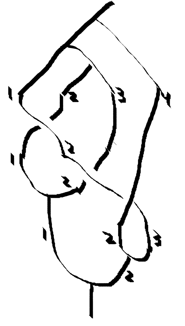
I started with the tree at the top and traversed downward implementing each braid and fusion. Implicitly all the particles shown in the diagram are Tau particles. The indices refer to particle position, not to the particles “identity” as you would trace it by eye on the page. Since these are identical quantum particles, the particles don’t have identity as we classically think of it anyhow.
The particle pairs are indexed by the number on the left particle. First braid 1 over 2, then 2 over 3, fuse 1 and 2, braid 2 under 3, fuse 2 and 3, and then fuse 1 and 2. I got an amplitude for the process of -0.618, corresponding to a probability of 0.382. I would give myself 70% confidence that I implemented all my signs and conventions correctly. The hexagon and pentagon equations from last time being correct gives me some peace of mind.
Syntax could use a little spit polish, but it is usable. With some readjustment, one could use the Haskell do notation removing the need for explicit >>=.
Next Time
Anyons are often described in categorical terminology. Haskell has a category culture as well. Let’s explore how those mix!