Variational Method of the Quantum Simple Harmonic Oscillator using PyTorch
A fun method (and useful!) for solving the ground state of the Schrodinger equation is to minimize the energy integral $ dx \psi^\dagger H \psi $ while keeping the total probability 1. Pytorch is a big ole optimization library, so let’s give it a go.
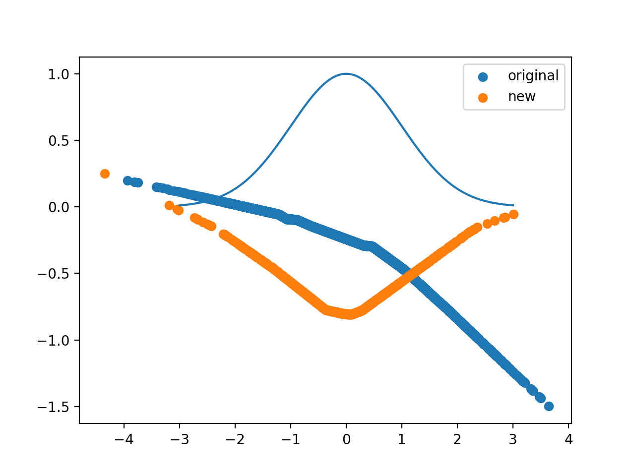
I’ve tried two versions, using a stock neural network with relus and making it a bit easier by giving a gaussian with variable width and shift.
We can mimic the probability constraint by dividing by to total normalization $ \int dx \psi^\dagger \psi$. A Lagrange multiplier or penalty method may allows us to access higher wavefunctions.
SGD seems to do a better job getting a rounder gaussian, while Adam is less finicky but makes a harsh triangular wavefunction.
The ground state solution of $ -\frac{d^2\psi}{dx^2} + x^2\psi=E\psi$ is $ e^{-x^2/2}$, with an energy of 1/2 (unless I botched up my head math). We may not get it, because we’re not sampling a very good total domain. Whatever, for further investigation.
Very intriguing is that pytorch has a determinant in it, I believe. That opens up the possibility of doing a Hartree-Fock style variational solution.
Here is my garbage
import torch
import matplotlib.pyplot as plt
import numpy as np
import torch.optim
from scipy import linalg
import time

import torch.nn as nn
import torch.nn.functional as F


class Psi(nn.Module):
    def __init__(self):
        super(Psi, self).__init__()

        # an affine operation: y = Wx + b
        self.lin1 = nn.Linear(1, 10) #Takes x to the 10 different hats
        self.lin2 = nn.Linear(10, 1) #add up the hats.
        #self.lin1 = nn.Linear(1, 1) #Takes x to the 10 different hats
        #self.lin2 = nn.Linear(2, 1) #add up the hats.
    def forward(self, x):
        # Max pooling over a (2, 2) window
        shifts = self.lin1(x)
        hats =  F.relu(shifts) #hat(shifts)hat(shifts)
        y = self.lin2(hats)
        #y = torch.exp(- shifts ** 2 / 4)
        return y


#a = torch.ones(10, requires_grad=True)
#z = torch.linspace(0, 1, steps=10)


# batch variable for monte carlo integration
x = torch.randn(10000,1, requires_grad=True) # a hundred random points between 0 and 1

psi = Psi()
y = psi(x)
import torch.optim as optim

# create your optimizer

optimizer =  optim.SGD(psi.parameters(), lr=0.0001, momentum=0.9, nesterov=True)
#optim.Adam(psi.parameters())
#optim.Adam(psi.parameters())
#y2 = torch.sin(np.pi*x)
#print(y)
#x2 = x.clone()
plt.scatter(x.detach().numpy(),y.detach().numpy(), label="original")
#plt.scatter(x.detach().numpy(),x.grad.detach().numpy())
scalar = torch.ones(1,1)
for i in range(4000):
    #print(x.requires_grad)
    #y.backward(torch.ones(100,1), create_graph=True)
    x = torch.randn(1000,1, requires_grad=True) # a hundred random points between 0 and 1


    y = psi(x)
    psi.zero_grad()

    y.backward(torch.ones(1000,1), create_graph=True)
    #torch.autograd.backward(torch.sum(y), grad_tensors=x)
    #print(x.grad)
    #print(dir(x)) #x.grad ** 2 +
    E = torch.sum(x.grad ** 2 + x**2 * y**2)#+ 10*(psi(scalar*0)**2 + psi(scalar)**2)
    N = torch.sum(y ** 2)
    L = E/N
    print(L)
    psi.zero_grad()
    L.backward()
    optimizer.step()
for param in psi.parameters():
    print(param)
    print(param.grad)
plt.scatter(x.detach().numpy(),y.detach().numpy(), label="new")
plt.legend()
#plt.scatter(x.detach().numpy(),x.grad.detach().numpy())
plt.show()

# may want to use the current wavefunction for gibbs style sampling
# we need to differentiate with respect to x for the kinetic energy
Edit: Hmm I didn’t compensate for the fact I was using randn sampling. That was a goof. I started using unifrom sampling, which doesn’t need compensation