The Classical Coulomb Gas as a Mixed Integer Quadratic Program
The coulomb gas is a model of electrostatics where you take the discreteness of charge into account. That is what makes it hard compared to the continuous charge problem. Previously, I’ve used mixed integer programming to find lowest energy states of the ising model. This is even more obvious application of mixed integer programming to a physics model.
We ordinarily consider electric charge to be a continuum, but it isn’t. It comes in chunks of the electron charge. Historically, people didn’t even know that for quite a while. It is usually a reasonable approximation for most purposes to consider electric charge to be continuous
If you consider a network of capacitors cooled to the the level that there is not enough thermal energy to borrow to get an electron to jump, the charges on the capacitors will be observably discretized. With a sufficiently slow cooling to this state, the charges should arrange themselves into the lowest energy state.
The coulomb gas model also is of interest due to its connections to the XY model, which I’ve taken a stab at with mixed integer programming before. The coulomb gas models the energy of vortices in that model. I think the connection between the models actually requires a statistical or quantum mechanical context though, whereas we’ve been looking at the classical energy minimization.
We can formulate the classical coulomb gas problem very straightforwardly as a mixed integer quadratic program. We can easily include an externally applied field and a charge conservation constraint if we so desire within the framework.
We write this down in python using the cvxpy library, which has a built in free MIQP solver, albeit not a very good one. Commercial solvers are probably quite a bit better.
import cvxpy as cvx
import numpy as np
#grid size
N = 5
# charge variables
q = cvx.Variable( N*N ,integer=True)

# build our grid
x = np.linspace(0,1,N)
y = np.linspace(0,1,N)
X, Y = np.meshgrid(x,y, indexing='ij')
x1 = X.reshape(N,N,1,1)
y1 = Y.reshape(N,N,1,1)
x2 = X.reshape(1,1,N,N)
y2 = Y.reshape(1,1,N,N)
eps = 0.1 / N #regularization factor for self energy. convenience mostly
V = 1. / ((x1-x2)**2 + (y1-y2)**2 + eps**2)** ( 1 / 2)
V = V.reshape( (N*N,N*N) )

U_external = 100 * Y.flatten() # a constant electric field in the Y direction
energy = cvx.quad_form(q,V) + U_external*q

# charge conservation constraint
prob = cvx.Problem(cvx.Minimize(energy),[cvx.sum(q)==0])
res = prob.solve(verbose=True)

print(q.value.reshape((N,N)))

#plotting junk

import matplotlib.pyplot as plt
from mpl_toolkits.mplot3d import Axes3D
fig = plt.figure()
ax = fig.add_subplot(111, projection='3d')

ax.plot_surface(X, Y, q.value.reshape((N,N)))
plt.show()
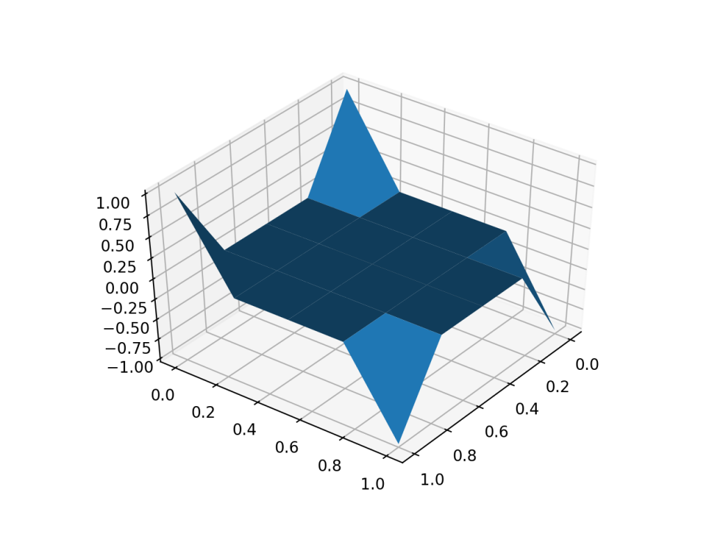 A plot of charge in a constant external electric field.
The results seems reasonable. It makes sense for charge to go in the direction of the electric field. Going to the corners makes sense because then like charges are far apart. So this might be working. Who knows.
Interesting places to go with this:
Prof Vanderbei shows how you can embed an FFT to enable making statements about both the time and frequency domain while keeping the problem sparse. The low time/memory $ N log(N) $ complexity of the FFT is reflected in the spasity of the resulting linear program.
https://vanderbei.princeton.edu/tex/ffOpt/ffOptMPCrev4.pdf
Here’s a sketch about what this might look like. Curiously, looking at the actual number of nonzeros in the problem matrices, there are way too many. I am not sure what is going on. Something is not performing as i expect in the following code
import cvxpy as cvx
import numpy as np
import scipy.fftpack # import fft, ifft
def swizzle(x,y):
    assert(x.size == y.size)
    N = x.size
    s =  np.exp(-2.j * np.pi * np.arange(N) / N)
    #print(s)
    #ret = cvx.hstack( [x + s*y, x - s*y])
    #print(ret.shape)
    return cvx.hstack( [x - s*y, x + s*y])


def fft(x):
    N = x.size
    #assert(2**int(log2(N)) == N) # power of 2

    if N == 1:
        return x, []
    else:
        y = cvx.reshape(x,(N//2,2))
        c = []
        even, ce = fft(y[:,0])
        c += ce
        odd, co = fft(y[:,1])
        c += co
        z = cvx.Variable(N, complex=True)
        c += [z == swizzle(even,odd)]
        return z, c

N = 256
x = cvx.Variable(N, complex=True)
z, c = fft(x)
v = np.zeros(N) #np.ones(N) #np.random.rand(N)
v[0]= 1
c += [x == v]
prob = cvx.Problem( cvx.Minimize(1), c)
#print(prob.get_problem_data(cvx.OSQP))
res = prob.solve(verbose=True)
#print(x.value)
print(z.value)
print(scipy.fftpack.fft(v))
print(scipy.fftpack.fft(v) - z.value)
The equivalent dense DFT:
x = cvx.Variable(N, complex=True)
fred = cvx.Variable(N, complex=True)
c = [fred == np.exp(-2.j * np.pi * np.arange(N).reshape((N,1)) * np.arange(N).reshape((1,N)) / N) * x]
prob = cvx.Problem( cvx.Minimize(1), c)
print(prob.get_problem_data(cvx.OSQP))
It would be possible to use a frequency domain solution of the interparticle energy rather than the explicit coulomb law form. Hypothetically this might increase the sparsity of the problem.
It seems very possible to me in a similar manner to embed a fast multipole method or barnes-hut approximation within a MIQP. Introducing explicit charge summary variables for blocks would create a sparse version of the interaction matrix. So that’s fun.