Some Notes on Drake: A Robotic Control ToolBox
Dumping these notes out there as is. Some material is out of date. Hope they’re useful.
What is Drake?
From the Drake Website (https://drake.mit.edu/):
“Drake (“dragon” in Middle English) is a C++ toolbox started by the Robot Locomotion Group at the MIT Computer Science and Artificial Intelligence Lab (CSAIL). The development team has now grown significantly, with core development led by the Toyota Research Institute. It is a collection of tools for analyzing the dynamics of our robots and building control systems for them, with a heavy emphasis on optimization-based design/analysis.
While there are an increasing number of simulation tools available for robotics, most of them function like a black box: commands go in, sensors come out. Drake aims to simulate even very complex dynamics of robots (e.g. including friction, contact, aerodynamics, …), but always with an emphasis on exposing the structure in the governing equations (sparsity, analytical gradients, polynomial structure, uncertainty quantification, …) and making this information available for advanced planning, control, and analysis algorithms. Drake provides interfaces to high-level languages (MATLAB, Python, …) to enable rapid-prototyping of new algorithms, and also aims to provide solid open-source implementations for many state-of-the-art algorithms. Finally, we hope Drake provides many compelling examples that can help people get started and provide much needed benchmarks. We are excited to accept user contributions to improve the coverage.”
Drake is a powerful toolkit for the control of dynamical systems, and I hope I lower some of the barrier to entry with this post. Be forewarned, Drake changes quickly with time, and some of the following may be out of date (especially the rigid body trees) or ill advised. Use your judgement.
Getting Drake
Drake may be installed from binaries or source. Both may be gotten here:
https://drake.mit.edu/installation.html
Using Bazel
Drake uses Bazel as a build tool. Bazel is an open-source build and test tool similar to Make, Maven, and Gradle.
There are three commands that you need to know:
bazel buildbazel runbazel query
Query is very useful for investigating available binaries within the examples folder and elsewhere.
The notation // is used to refer to the build’s main directory. This corresponds to the drake folder.
... is the notation for everything in the subdirectory
Examples:
bazel build //...will build everything in the project.- To query all the binaries available for tools run
bazel query //tools/...
Using Pydrake
Drake can be run natively in C++, or by using its MATLAB, python, or Julia bindings. This manual will be focusing on using Drake in python. By default pydrake will not be in the path. You can put pydrake into the path after building by running the following line or adding it to your .bashrc
export PYTHONPATH=~/drake/drake-build/install/lib/python2.7/site-packages:${PYTHONPATH}
The following line will import everything in Drake into the python namespace.
from pydrake.all import *
Drake is only compatible with python 2.7. If your default system install is python3, you may need to explicitly run the command python2.
The following message may be thrown if you inadvertently use python3.
Traceback (most recent call last):
File "inverse_kinematics.py", line 2, in <module>
from pydrake.all import

...

ImportError: dynamic module does not define module export function (PyInit__common_py)
Pydrake itself has generated documentation available here:
http://drake.mit.edu/pydrake/index.html
This is an extremely useful resource.
A very useful tool for exploring and confirming the Drake functionality and syntax is the python REPL. From the python REPL or within your code, it is useful to inspect an object using either help(obj) or print(dir(obj)) which will print a list of all the properties available on your object.
Drake resources
Doxygen
Besides the source code itself, the most accurate and up to date information is available in searchable form on the Doxygen page. This is a useful reference, but can be overwhelming.
https://drake.mit.edu/doxygen_cxx/index.html
Underactuated Robotics textbook and examples
Drake has a textbook being built alongside it by Russ Tedrake.
http://underactuated.mit.edu/underactuated.html
In particular the python source used to generate some of the examples in the book is worth examining.
https://github.com/RussTedrake/underactuated/tree/master/src
The full course is available online both on Edx and more recent versions on Youtube.
http://underactuated.csail.mit.edu/Spring2018/
Examples directory.
A useful source of use cases for drake can be found in the examples directory within the Drake project. As of October 2018 the contents include:
- Cartpole - The cartpole is a classic control system consisting of a pendulum attached to a linearly actuated cart. In this directory you can find examples
- Pendulum
- Double Pendulum
- Acrobot - The Acrobot is a double pendulum system actuated at the shoulder
- Kinova Jaco Arm - A commercially available robotic arm
- Kuka Iiwa Arm - A commerically available robotic arm
- Particles
- Bouncing Ball
- Contact Model - Contains bowling pins, a gripper, and sliding bricks demonstrating Drakes ability to simulate contact dynamics
- Rimless Wheel - A very simple model of a walking robot
- Compass Gait - A slightly less simple model of a walking robot
- Atlas - Examples concerning the Atlas humanoid robot
- zmp
- quadcopter
- and others
Additional usage examples for pydrake can be found in the drake/bindings/pydrake/test folder.
Periscope Tutorials
There is a set of Jupyter notebook based tutorials for some basic Drake functionality in python.
https://github.com/gizatt/drake_periscope_tutorial
Drake Concepts
Simulation
For dynamic simulation, Drake exposes a Lego block interface for building complex systems out of smaller pieces, a paradigm similar to Simulink and other modeling software.
Objects possess input and output ports. One wires up input ports to output ports to build composite systems.
To build a simple forward simulation, construct a builder object. Then add all subsystems to the builder object. Explicitly connected input and output ports together. One possible cause of crashes may be leaving ports unconnected.
Once the entire system has been built, a Simulator object can be constructed from it. You may select an integration scheme and set initial conditions by getting a context from the Simulator object. The context holds state information.
There following excerpt from https://github.com/RussTedrake/underactuated/tree/master/src/simple shows how to define a simple system and simulate it.
from pydrake.systems.framework import VectorSystem

# Define the system.
class SimpleContinuousTimeSystem(VectorSystem):
def __init__(self):
VectorSystem.__init__(self,
0, # Zero inputs.
1) # One output.
self._DeclareContinuousState(1) # One state variable.

# xdot(t) = -x(t) + x^3(t)
def _DoCalcVectorTimeDerivatives(self, context, u, x, xdot):
xdot[:] = -x + x**3

# y(t) = x(t)
def _DoCalcVectorOutput(self, context, u, x, y):
y[:] = x
import matplotlib.pyplot as plt
from pydrake.all import (DiagramBuilder, SignalLogger, Simulator)
from continuous_time_system import *

# Create a simple block diagram containing our system.
builder = DiagramBuilder()
system = builder.AddSystem(SimpleContinuousTimeSystem())
logger = builder.AddSystem(SignalLogger(1))
builder.Connect(system.get_output_port(0), logger.get_input_port(0))
diagram = builder.Build()

# Create the simulator.
simulator = Simulator(diagram)

# Set the initial conditions, x(0).
state = simulator.get_mutable_context().get_mutable_continuous_state_vector()
state.SetFromVector([0.9])

# Simulate for 10 seconds.
simulator.StepTo(10)

# Plot the results.
plt.plot(logger.sample_times(), logger.data().transpose())
plt.xlabel('t')
plt.ylabel('x(t)')
plt.show()
Refs:
http://underactuated.mit.edu/underactuated.html?chapter=systems
Rigid Body Trees
Edit : I think the Rigid Body Trees interface is deprecated. Use Multi Body Trees.
There are two complementary perspectives to take of the degrees of freedom of a robot, intrinsic coordinates and extrinsic coordinates. The intrinsic coordinates have one variable per degree of freedom of the robot. A common example is a set of joint angles. The dynamics are simply expressed in the intrinsic coordinates and can derived using Lagrangian mechanics. The extrinsic coordinates specify the spatial locations and orientation of frames attached to the robot. These are called frames. These spatial coordinates may be constrained in a relationship by a rigid mounting or gearing, so there may be more extrinsic frames available than intrinsic coordinates. Extrinsic coordinates are particularly pertinent for discussions of geometry, contact, and external forces.
Drake uses the URDF (Universal Robot Description Format) format. This is a common robot format originating in the ROS community for which you can find models of many commercial robots online. It is an XML based format with visualization, inertial, and collision tags.

This is an example URDF for a pendulum cart system.
Example: Pendulum URDF
<robot xmlns:xsi="http://www.w3.org/2001/XMLSchema-instance" xmlns="http://drake.mit.edu" name="CartPole">

    <link name="ground">
        <visual>
            <origin rpy="0 0 0" xyz="0 0 -5"></origin>
            <geometry>
                <box size="1000 1000 10"></box>
            </geometry>
            <material>
                <color rgba="0.93 .74 .4 1"></color>
            </material>
        </visual>
    </link>

    <link name="cart">
        <inertial>
            <origin rpy="0 0 0" xyz="0 0 -.5"></origin>
            <mass value="10"></mass>
            <inertia ixz="0" ixx="0" ixy="0" izz="0" iyy="0" iyz="0"></inertia>
        </inertial>
        <visual>
            <origin rpy="0 0 0" xyz="0 0 .25"></origin>
            <geometry>
                <box size=".6 .3 .3"></box>
            </geometry>
            <material>
                <color rgba="0 1 0 1"></color>
            </material>
        </visual>
        <visual>
            <origin rpy="0 0 0" xyz=".15 0 .025"></origin>
            <geometry>
                <sphere radius=".05"></sphere>
            </geometry>
            <material>
                <color rgba="0 0 0 1"></color>
            </material>
        </visual>
        <visual>
            <origin rpy="0 0 0" xyz="-.15 0 .025"></origin>
            <geometry>
                <sphere radius=".05"></sphere>
            </geometry>
            <material>
                <color rgba="0 0 0 1"></color>
            </material>
        </visual>
    </link>

    <link name="pole">
        <inertial>
            <origin rpy="0 0 0" xyz="0 0 -.5"></origin>
            <mass value="1"></mass>
            <inertia ixz="0" ixx="0" ixy="0" izz="0" iyy="0" iyz="0"></inertia>
        </inertial>
        <visual>
            <origin rpy="0 0 0" xyz="0 0 -.25"></origin>
            <geometry>
                 <cylinder length=".5" radius=".01"></cylinder>
            </geometry>
            <material>
                <color rgba="1 0 0 1"></color>
            </material>
        </visual>
        <visual>
            <origin rpy="0 0 0" xyz="0 0 -.5"></origin>
            <geometry>
                 <sphere radius=".05"></sphere>
            </geometry>
            <material>
                <color rgba="0 0 1 1"></color>
            </material>
        </visual>
    </link>

    <joint type="prismatic" name="x">
        <parent link="ground"></parent>
        <child link="cart"></child>
        <origin xyz="0 0 0"></origin>
        <axis xyz="1 0 0"></axis>
        <dynamics damping="0.1"></dynamics>
    </joint>

    <joint type="continuous" name="theta">
        <parent link="cart"></parent>
        <child link="pole"></child>
        <origin xyz="0 0 .25"></origin>
        <axis xyz="0 1 0"></axis>
        <dynamics damping="0.1"></dynamics>
    </joint>

    <transmission type="SimpleTransmission" name="cart_force">
        <actuator name="force"></actuator>
        <joint name="x"></joint>
        <mechanicalreduction>1</mechanicalreduction>
    </transmission>
</robot>
Ref:
https://github.com/RussTedrake/underactuated/blob/master/src/cartpole/cartpole.urdf
The RigidBodyTree is a Drake class that describes both the intrinsic and extrinsic properties of a linkage. RigidBodyTrees may be built from a URDF file, some of which are packaged inside of Drake. For example, the Jaco arm URDF is available packaged with Drake.
jaco_urdf = FindResourceOrThrow(
    "drake/manipulation/models/jaco_description/urdf/j2n6s300.urdf")
tree = RigidBodyTree(jaco_urdf, FloatingBaseType.kFixed)
The full properties of the RigidBodyTree class are available at https://drake.mit.edu/pydrake/pydrake.multibody.rigid_body_tree.html , but it will be useful to highlight some of the most commonly used functionality.
You can probe the RigidBodyTree for useful properties about the linkage, for example the number of intrinsic coordinates, or the number of bodies in the tree.
print(tree.get_num_positions())
print(tree.get_num_velocities())
print(tree.get_num_bodies())
For many operations, one needs to perform the forward dynamics to build a kinematic cache that needs to be supplied later.
q = np.zeros(tree.get_num_positions())
v = np.zeros(tree.get_num_velocities())
cache = tree.doKinematics(q,v)
Drake describes the dynamics in terms of the intrinsic coordinates. The robot manipulator equations have the common form (See http://underactuated.csail.mit.edu/underactuated.html?chapter=multibody )
$ M(q)\ddot{q} + C(q,\dot{q})\dot{q} = \tau_g(q) + Bu $
where q is the state vector, M is the inertia matrix, C captures Coriolis forces, and $ \tau_g$ is the gravity vector. The matrix B maps control inputs u into generalized forces.
External forces on the tree are described as wrenches. Wrenches are an object that combines forces and torques. In Drake, they are specified by 6 dimensional vectors. From the Drake docs:
“A column vector consisting of one wrench (spatial force) = [r X f; f], where f is a force (translational force) applied at a point P and r is the position vector from a point O (called the “moment center”) to point P.”
Drake will also compute the quantities in the manipulator equation. For example, to compute the term $ C(q,v,f_{ext})$ in the manipulator equations with no externally applied wrenches.
bodies = [tree.get_body(j) for j in range(tree.get_num_bodies())]
no_wrench = { body : np.zeros(6) for body in bodies}
print(tree.dynamicsBiasTerm(cache, no_wrench))
Drake can be asked to compute the other terms in the manipulator equation as well. Drake can compute the center of mass of the entire tree.
tree.centerOfMass(cache)
Drake provides a couple of useful mappings between the intrinsic and extrinsic coordinates.
First, given a set of internal coordinates, Drake can transform these into frames, which may be expressed in yet another coordinate system.
The extrinsic frames can be expressed as a function of the intrinsic coordinates
$ X_i = f_i(x_j) $
tree.relativeTransform(cache, 0, 9)
Returns a $ 4\times 4$ transformation matrix between body 0 and 9 of the tree. The upper $ 3\times 3$ block corresponds to a rotation matrix, and the last column a translation vector of the frame.
The Jacobian of this mapping,
$ J_{ij} = \frac{\partial f_i}{\partial x_j} $
is useful for translating externally described small displacements, velocities, forces, and torques, into the equivalent terms for the intrinsic coordinates.
The time derivative or differential of a frame will possess a linear and angular velocity. These come packed in a 6 dimensional vector called the Twist.
https://en.wikipedia.org/wiki/Screw_theory#Twist
The geometric Jacobian function returns the Jacobian in a sparse format. It returns a tuple of a $ m\times 6$ matrix and a $ 1\times m$ vector of indices to which coordinates these correspond.
The function takes the id of three different frames. In this example, it computes the differential of the transformation from frame 0 to frame 9 expressed in frame 3.
tree.geometricJacobian(cache, 0, 9, 3)
The dense matrix can be constructed by
jsparse, inds = tree.geometricJacobian(cache, 0, 9, 0)
jdense = np.zeros((tree.get_num_positions(), 6))
jdense[inds, :] = jsparse
Refs:
A Mathematical Introduction to Robotic Manipulation - https://www.cds.caltech.edu/~murray/books/MLS/pdf/mls94-complete.pdf
http://underactuated.csail.mit.edu/underactuated.html?chapter=intro
Visualization
The Drake visualizer may be found in the tools folder. The Drake visualizer needs to be running before any applications that needs to communicate with it are started. To get the drake visualizer running run the following command from the drake directory
bazel run //tools:drake_visualizer
May need to run commands here to make LCM work and visualizer not crash immediately
http://lcm-proj.github.io/multicast_setup.html
sudo ifconfig lo multicast
sudo route add -net 224.0.0.0 netmask 240.0.0.0 dev lo
Kinova ROS package
The Kinova Jaco arm is easily communicated to through the Kinova ROS package
https://github.com/Kinovarobotics/kinova-ros
The package as of October 2018 supports Ubuntu 14.04 and ROS Indigo. The package includes bindings to the Jaco SDK for reading sensor data and giving motion commands. The package supports a variety of control modes, including torque control.
To update functionality to ubuntu 16.04 and ROS Kinetic you may wish to pull from this external branch
https://github.com/CNURobotics/kinova-ros/tree/kinetic_devel
or try the beta branch
https://github.com/Kinovarobotics/kinova-ros/tree/kinova-ros-beta
The Gazebo simulator seems to have a great deal of trouble.
One suggestion is that you have to add a small nonzero size parameter to your URDF files. https://github.com/Kinovarobotics/kinova-ros/issues/103
The topics made available by the ROS Package are
/j2n6s300_driver/fingers_action/finger_positions/cancel
/j2n6s300_driver/fingers_action/finger_positions/feedback
/j2n6s300_driver/fingers_action/finger_positions/goal
/j2n6s300_driver/fingers_action/finger_positions/result
/j2n6s300_driver/fingers_action/finger_positions/status
/j2n6s300_driver/in/cartesian_force
/j2n6s300_driver/in/cartesian_velocity
/j2n6s300_driver/in/joint_torque
/j2n6s300_driver/in/joint_velocity
/j2n6s300_driver/joints_action/joint_angles/cancel
/j2n6s300_driver/joints_action/joint_angles/feedback
/j2n6s300_driver/joints_action/joint_angles/goal
/j2n6s300_driver/joints_action/joint_angles/result
/j2n6s300_driver/joints_action/joint_angles/status
/j2n6s300_driver/out/cartesian_command
/j2n6s300_driver/out/finger_position
/j2n6s300_driver/out/joint_angles
/j2n6s300_driver/out/joint_command
/j2n6s300_driver/out/joint_state
/j2n6s300_driver/out/joint_torques
/j2n6s300_driver/out/tool_pose
/j2n6s300_driver/out/tool_wrench
/j2n6s300_driver/pose_action/tool_pose/cancel
/j2n6s300_driver/pose_action/tool_pose/feedback
/j2n6s300_driver/pose_action/tool_pose/goal
/j2n6s300_driver/pose_action/tool_pose/result
/j2n6s300_driver/pose_action/tool_pose/status
/j2n6s300_driver/trajectory_controller/command
/j2n6s300_driver/trajectory_controller/state
ROS Intercommunication
The communication stack used by Drake is Lightweight Communications and Marshalling (LCM). For interconnection to the rest of the ROS ecosystem, this adds a layer of friction.
One option is to use the lcm_to_ros project https://github.com/nrjl/lcm_to_ros
This is a generator for building republishers of messages going between ROS and LCM
Another option is to build custom subscribers and publishers as in the following example.
http://wiki.ros.org/ROS/Tutorials/WritingPublisherSubscriber%28python%29
Example: Connecting Drake Visualizer to External Jaco Arm
In another terminal turn on the Jaco driver
roslaunch kinova_bringup kinova_robot.launch kinova_robotType:=j2n6s300
Also get the drake visualizer running from the drake directory before running the script
bazel run //tools:drake_visualizer
import rospy
from pydrake.all import *
import numpy as np
from sensor_msgs.msg import JointState
jaco_urdf = FindResourceOrThrow("drake/manipulation/models/jaco_description/urdf/j2n6s300.urdf")
tree = RigidBodyTree(jaco_urdf , FloatingBaseType.kFixed)

builder = DiagramBuilder()

lc = DrakeLcm()
vis = DrakeVisualizer(tree, lc)
robot = builder.AddSystem(RigidBodyPlant(tree))
publisher = builder.AddSystem(vis)
builder.Connect(robot.get_output_port(0), publisher.get_input_port(0))

diagram = builder.Build()
simulator = Simulator(diagram)
simulator.set_target_realtime_rate(1.0)
simulator.set_publish_every_time_step(False)
context = simulator.get_mutable_context()
state = context.get_mutable_continuous_state_vector()
state.SetFromVector(np.zeros(9*2))
simulator.Initialize()


q = None
v = None
f = None
def callback(data):
        global q, v, f
        q = np.array(data.position)
        v = np.array(data.velocity)
        f = np.array(data.effort)
        # Some of the coordinates are offset between the Kinova Ros package and the Drake model
        q[1] = np.pi + q[1]
        q[2] = np.pi + q[2]


rospy.init_node('listener', anonymous=True)
rospy.Subscriber("/j2n6s300_driver/out/joint_state", JointState, callback)

rate = rospy.Rate(4)
rate.sleep()
while not rospy.is_shutdown():
        state = context.get_mutable_continuous_state_vector()
        state.SetFromVector(np.append(q,v))
        simulator.Initialize()
        rate.sleep()

Example: Crumpling Jaco
A simple example of the simulation capabilities is the simulation of an unactuated Jaco arm.
import rospy
from pydrake.all import *
import numpy as np
from sensor_msgs.msg import JointState
jaco_urdf = FindResourceOrThrow("drake/manipulation/models/jaco_description/urdf/j2n6s300.urdf")
tree = RigidBodyTree(jaco_urdf , FloatingBaseType.kFixed)

builder = DiagramBuilder()

lc = DrakeLcm()
vis = DrakeVisualizer(tree, lc)
robot = builder.AddSystem(RigidBodyPlant(tree))
publisher = builder.AddSystem(vis)
builder.Connect(robot.get_output_port(0), publisher.get_input_port(0))
force = builder.AddSystem(ConstantVectorSource(np.zeros(9)))
builder.Connect(force.get_output_port(0), robot.get_input_port(0))

diagram = builder.Build()
simulator = Simulator(diagram)
simulator.set_target_realtime_rate(1.0)
simulator.set_publish_every_time_step(False)
context = simulator.get_mutable_context()
state = context.get_mutable_continuous_state_vector()
state.SetFromVector(np.zeros(9*2)+0.1)
simulator.Initialize()
simulator.StepTo(10)
Optimization Solvers
Drake provides a common interface to many optimization solvers. Because of the tight integration, Drake has the capability to directly build the equations of motion for a system into a form the solver can comprehend.
The Mathematical Program class provides a high level interface to the different solvers. This class can be constructed as an object on it’s own or as returned by other helper classes such as trajectory optimization builders.
Drake provides a symbolic expression modeling language in which to describe constraints and costs.
from pydrake.all import *
import numpy as np

m = MathematicalProgram()

xs = m.NewContinuousVariables(2, 'x')
print(xs)
c = np.array([-1,-1])
m.AddCost( c[0]*xs[0] + c[1]*xs[1] )

m.AddLinearConstraint(xs[0] == 0)
m.AddLinearConstraint(3*xs[1] + xs[0] <= -1)

print(m.linear_equality_constraints())
print(m.bounding_box_constraints())
print(m.linear_costs()[0])
print(m.Solve())
print(m.GetSolverId().name())
print(m.GetSolution(xs))
There are a large variety of solvers out there for problems of different structure.
A Mathematical Program is generally of the form
$ \min f(x) \ s.t. $
$ g(x) \ge 0 $
$ h(x) = 0 $
One of the oldest and most studied class of these programs are known as Linear Programs which has linear cost and constraints. This mathematical program has very efficient solvers available for it.
A large class of optimization problems that are tractable are known as Convex Optimization problems. The cost functions must be bowl shaped (convex), the inequality constraints must define convex regions and the equality constraints must be affine (linear + offset). For this class, gradient descent roughly works and refinements of gradient descent like Newton’s method work even better. Convexity implies that greedy local moves are also acceptable global moves and there are no local minima or tendril regions to get caught in.
The common reference for convex optimization is the textbook by Boyd and Vandenberghe freely available at http://web.stanford.edu/~boyd/cvxbook/. There is also an accompanying video course available online.
Subclasses of Convex programming may have solvers tuned to them. Important subclasses include:
- Linear Programming - Linear objective, linear equality, and linear inequality constraints.
- Quadratic Programming - Linear Programming + quadratic objective
- Second Order Cone Programming
- Semidefinite Programming - Optimization allowing for the constraint of a SemiDefinite matrix. This means the matrix is constrained to have all nonnegative eigenvalues or equivalently the quadratic form it defines $ q^T Xq$ is non-negative for all possible vectors $ q$.
- Sum of Squares Programming - Optimization over polynomials with the constraint that the polynomial can be written as a sum of squares, a manifestly positive form.
Many problems cannot be put into this form. If the inherent nature of the problem at hand requires it, you may choose to use a nonlinear programming solver or Mixed Integer Programming Solver.
The solvers Ipopt and Snopt are nonlinear programming solvers. Ipopt is an open source and Snopt is proprietary. These solvers use local convex approximations to the problem to heuristically drive the solution to a local minimum.
Mixed Integer Linear Programming is Linear Programming with additional ability to require variables to take on integer values. This additional constraint type takes the problem from polynomial time solvable to NP-complete. A surprisingly large number of discrete and continuous optimization problems can be encoded into this framework. Internally, these solvers use linear programming solvers to guide the discrete search.
Part of the art and fun of the subject comes from manipulating your problem into a form amenable to powerful available solvers and theory.
Hans Mittelmann at the University of Arizona maintains benchmarks for a variety of optimization tools. http://plato.asu.edu/bench.html A rule of thumb is that commercial solvers perform better than open source solvers.
Available Solvers in Drake
-
Mosek - Mosek is a proprietary optimization solver package offering solvers for
- Linear.
- Conic quadratic.
- Semi-definite (Positive semi-definite matrix variables).
- Quadratic and quadratically constrained.
- General convex nonlinear.
- Mixed integer linear, conic and quadratic.
-
Gurobi - Gurobi is a proprietary optimization solver package offering solvers for
- linear programming solver (LP)
- mixed-integer linear programming solver (MILP)
- mixed-integer quadratic programming solver (MIQP)
- quadratic programming solver (QP)
- quadratically constrained programming solver (QCP)
- mixed-integer quadratically constrained programming solver (MIQCP)
- Snopt - Snopt is a nonlinear optimization solver using sequential convex optimization (SQP) http://www.sbsi-sol-optimize.com/asp/sol_product_snopt.htm
- Ipopt - Ipopt is a open source nonlinear optimization solver using sequential convex optimization (SQP) https://projects.coin-or.org/Ipopt
- Operator Splitting Quadratic Program (OSQP) - Open source quadratic programming package https://osqp.org/
- ik
- LCP
- dReal - An SMT solver for reals http://dreal.github.io/
Automatic Differentiation
Automatic Differentiation is the capability to have derivatives computed alongside code that computes the values. It is largely based upon application of the chain rule. There are two modes, forward and reverse mode.
Forward mode is the simplest to describe. Functions can be overloaded so that they take a dual number, a value combined in a tuple with it’s derivative information. As the value of a function is computed, the Jacobian of that function is matrix multiplied on the derivative concurrently.
Drake exposes automatic differentiation capability for manual use
from pydrake.all import *
import numpy as np

# second parameter initializes forward mode derivative information
x = AutoDiffXd(4.0, np.array([1,1]))
f = x * x * x
print(f.derivatives())
More importantly Drake uses automatic differentiation internally to marshal symbolic problems into forms acceptable to external solvers and to calculate the various Jacobians we’ve already seen.
Trajectory Optimization
Trajectory optimization is a framework in which one uses Mathematical programming to solve optimal trajectory problems. The input to the system
is considered to be a decision variable in a Mathematical programming problem.
The combination of dynamical system modeling, automatic differentiation, and bindings to mathematical programming solvers makes Drake an excellent platform for trajectory optimization.
In Direct Collocation, both the path and the input variables are discretized along time. The trajectories are described by cubics and force curves are described by piecewise linear. One way of performing direct collocation is to take the path position at a discrete number of time points and make a decision variable for each. The discretized equations of motion become constraints that neighboring time points have to obey. One may then inject any other desired requirements (staying inside some safe region for example) as additional constraints.
The Drake docs state:
”
DirectCollocation implements the approach to trajectory optimization as described in C. R. Hargraves and S. W. Paris. Direct trajectory optimization using nonlinear programming and collocation. J Guidance, 10(4):338-342, July-August 1987. It assumes a first-order hold on the input trajectory and a cubic spline representation of the state trajectory, and adds dynamic constraints (and running costs) to the midpoints as well as the knot points in order to achieve a 3rd order integration accuracy.
”
Drake provides a useful interface for talking about trajectories. For both describing the cost function and the constraint functions, you want them to apply at all time steps. You can ask drake for variables representing the position or forces at all time steps. Drake will then build the appropriate mathematical program applying the cost of constraint at all time steps.
ctx = robot.CreateDefaultContext()
dircol = DirectCollocation(robot, ctx, 10, 0.01, 0.1) # timesteps, minimum time step, max timestep
dircol.AddEqualTimeIntervalsConstraints()

state = dircol.state
u = dircol.input
t = dircol.time

dircol.AddRunningCost(state[0]**2)
dircol.AddConstraintToAllKnotPoints(u[0] >= 0)
You may want to select the initial and final state specifically to specify goals and initial conditions
init = dircol.initial_state
final = dircol.final_state
Refs:
http://underactuated.mit.edu/underactuated.html?chapter=trajopt
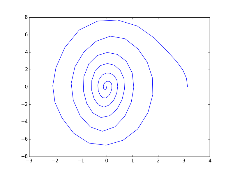
Example: Trajectory Optimization of a Pendulum
This example comes from the Underactuated Robotics textbook source
import math
import numpy as np
import matplotlib.pyplot as plt

from pydrake.examples.pendulum import (PendulumPlant, PendulumState)
from pydrake.all import (DirectCollocation, PiecewisePolynomial,
                                                 SolutionResult)
#from visualizer import PendulumVisualizer

plant = PendulumPlant()
context = plant.CreateDefaultContext()

dircol = DirectCollocation(plant, context, num_time_samples=21,
                            minimum_timestep=0.2, maximum_timestep=0.5)

dircol.AddEqualTimeIntervalsConstraints()

torque_limit = 3.0  # N*m.
u = dircol.input()
dircol.AddConstraintToAllKnotPoints(-torque_limit <= u[0])
dircol.AddConstraintToAllKnotPoints(u[0] <= torque_limit)

initial_state = PendulumState()
initial_state.set_theta(0.0)
initial_state.set_thetadot(0.0)
dircol.AddBoundingBoxConstraint(initial_state.get_value(),
                            initial_state.get_value(),
                            dircol.initial_state())
# More elegant version is blocked on drake #8315:
# dircol.AddLinearConstraint(dircol.initial_state()
#                               == initial_state.get_value())

final_state = PendulumState()
final_state.set_theta(math.pi)
final_state.set_thetadot(0.0)
dircol.AddBoundingBoxConstraint(final_state.get_value(),
                                final_state.get_value(),
                                dircol.final_state())
# dircol.AddLinearConstraint(dircol.final_state() == final_state.get_value())

R = 10  # Cost on input "effort".
dircol.AddRunningCost(R*u[0]**2)

initial_x_trajectory = \
        PiecewisePolynomial.FirstOrderHold([0., 4.],
                                 [initial_state.get_value(),
                                 final_state.get_value()])
dircol.SetInitialTrajectory(PiecewisePolynomial(),
                            initial_x_trajectory)
result = dircol.Solve()
assert(result == SolutionResult.kSolutionFound)
x_trajectory = dircol.ReconstructStateTrajectory()
#vis = PendulumVisualizer()
#ani = vis.animate(x_trajectory, repeat=True)
x_knots = np.hstack([x_trajectory.value(t) for t in
                      np.linspace(x_trajectory.start_time(),
                      x_trajectory.end_time(), 100)])
plt.figure()
plt.plot(x_knots[0, :], x_knots[1, :])
plt.show()
Example Application: Estimating end-effector force from Jaco motor torques
End effector forces become part of the equations of motion.
The geometric Jacobian transforms the extrinsic force into intrinsic coordinates. It is in general a rectangular matrix, since the number of extrinsic coordinates does not need to match the number of intrinsic coordinates.
A force $ f$ applied to the end effector appears linearly in the manipulator equations as $ J^Tf$. This will be canceled by the torques of the motors during static or quasi-static movement. Hence, we can can determinethe external force from the motor torques if we assume it is the only external force at play.
The pseudo-inverse is the best possible solution to an overdetermined set of linear equations, in the least squares sense. We use this operation due to the non square nature of the Jacobian.
$ \min (Jx - X)^2 \rightarrow J^T Jx = J^T X$
The following script prints both the end effector force as supplied by the Jaco SDK and the force as computed by Drake from the internal motor torques.
import rospy
from pydrake.all import *
import numpy as np
from sensor_msgs.msg import JointState
from geometry_msgs.msg import WrenchStamped
urdf_tree = FindResourceOrThrow("drake/manipulation/models/jaco_description/urdf/j2n6s300.urdf")
tree = RigidBodyTree( urdf_tree,
                                         FloatingBaseType.kFixed)
bodies = [tree.get_body(j) for j in range(tree.get_num_bodies())]
no_wrench = { body : np.zeros(6)  for body in bodies}

body_n = 9 #end_effector body number
print(bodies[body_n].get_name())

def end_effector_force(q, v, u):
        cache = tree.doKinematics(q,v)
        # returns the external torque term for only gravity and no other external wrenches
        Cgrav = tree.dynamicsBiasTerm(cache, no_wrench )
        C = u - Cgrav # subtract off gravity of robot itself
        print(u - Cgrav)
        j = tree.geometricJacobian(cache, 0 , body_n, 0) # returns a tuple of 6 by n matrix in j[0] and the indices to which it applied in j[1]
        jjt = np.dot(j[0] ,j[0].T) #
        Wext = np.linalg.solve(jjt,  np.dot(j[0],  C[j[1]])) # C[j[1]] is cryptic numpy sub indexing for densifying the Jacobian
        return Wext[3:]


q = None
v = None
f = None
fext = np.zeros(3)

def callback(data):
        global q, v, f, initu, start
        q = np.array(data.position)
        v = np.array(data.velocity)
        q[1] = np.pi + q[1] #The drake conventions and the kinova conventions for angles are off
        q[2] = np.pi + q[2]
        f = np.array(data.effort)

def wrenchcallback(data):
        global fext
        fext[0] = data.wrench.force.x
        fext[1] = data.wrench.force.y
        fext[2] = data.wrench.force.z

rospy.init_node('listener', anonymous=True)
rospy.Subscriber("/j2n6s300_driver/out/joint_state", JointState, callback)
rospy.Subscriber("/j2n6s300_driver/out/tool_wrench", WrenchStamped, wrenchcallback)

rate = rospy.Rate(1)
rate.sleep()
while not rospy.is_shutdown():
        print(end_effector_force(q,v,f))
        print(fext)
        rate.sleep()