Solving the XY Model using Mixed Integer Optimization in Python
There are many problems in physics that take the form of minimizing the energy. Often this energy is taken to be quadratic in the field. The canonical example is electrostatics. The derivative of the potential $ \phi$ gives the electric field E. The energy is given as $ \int (|\nabla \phi|^2 + \phi \rho) d^3 x $. We can encode a finite difference version of this (with boundary conditions!) directly into a convex optimization modelling language like so.
import cvxpy as cvx
import numpy as np
import matplotlib.pyplot as plt
import scipy.linalg
from mpl_toolkits import mplot3d


N = 10

# building a finite difference matrix. It is rectangle of size N x (N-1). It maps from the vertices of our grid to the lines in between them, where derivatives live.
col = np.zeros(N)
col[0] = -1
col[1] = 1
delta = scipy.linalg.toeplitz(col, np.zeros(N-1)).T
print(delta)

gradx = np.kron(delta, np.eye(N))
grady = np.kron(np.eye(N), delta)

# a variable for our potential
phi = cvx.Variable((N, N))

# vectorization is useful. It flattens out the x-y 2Dness.
phivec = cvx.vec(phi)
gradxvec = gradx.reshape(-1, N*N)
gradyvec = grady.reshape(-1, N*N)

V = cvx.sum_squares(gradxvec * phivec) + cvx.sum_squares(gradyvec * phivec)

constraints = []
# boundary conditions. Dirichlet
constraints += [phi[:,0] == 0, phi[0,:] == 0, phi[:,-1] == 0, phi[-1,:] == 0 ]

# fixed charge density rho
rho = np.zeros((N,N))
rho[N//2,N//2] = 1
print(rho)

# objective is energy
objective = cvx.Minimize(V + cvx.sum(cvx.multiply(rho,phi)))
prob = cvx.Problem(objective, constraints)
res = prob.solve()
print(res)
print(phi.value)

# Plotting
x = np.linspace(-6, 6, N)
y = np.linspace(-6, 6, N)

X, Y = np.meshgrid(x, y)
fig = plt.figure()

ax = plt.axes(projection='3d')
ax.plot_surface(X, Y, phi.value, rstride=1, cstride=1,
                cmap='viridis', edgecolor='none')
plt.show()
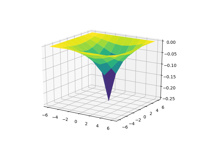 The resulting logarithm potential
It is noted rarely in physics, but often in the convex optimization world that the barrier between easy and hard problems is not linear vs. nonlinear, it is actually more like convex vs. nonconvex. Convex problems are those that are bowl shaped, on round domains. When your problem is convex, you can’t get caught in valleys or on corners, hence greedy local methods like gradient descent and smarter methods work to find the global minimum. When you differentiate the energy above, it results in the linear Laplace equations $ \nabla^2 \phi = \rho$. However, from the perspective of solvability, there is not much difference if we replace the quadratic energy with a convex alternative.
def sum_abs(x):
    return cvx.sum(cvx.abs(x))
V = cvx.sum_squares(gradxvec * phivec) + cvx.sum_squares(gradyvec * phivec)
V = cvx.sum(cvx.huber(gradxvec * phivec)) + cvx.sum(cvx.huber(gradyvec * phivec))
V = cvx.pnorm(gradxvec * phivec, 3) + cvx.pnorm(gradyvec * phivec, 3)

a = 1
dxphi = gradxvec * phivec
dyphi = gradyvec * phivec
V = cvx.sum(cvx.maximum( -a - dxphi, dxphi - a, 0 )) + cvx.sum(cvx.maximum( -a - dyphi, dyphi - a, 0 ))
Materials do actually have non-linear permittivity and permeability, this may be useful in modelling that. It is also possible to consider the convex relaxation of truly hard nonlinear problems and hope you get the echoes of the phenomenology that occurs there.
Another approach is to go mixed integer. Mixed Integer programming allows you to force that some variables take on integer values. There is then a natural relaxation problem where you forget the integer variables have to be integers. Mixed integer programming combines a discrete flavor with the continuous flavor of convex programming. I’ve previously shown how you can use mixed integer programming to find the lowest energy states of the Ising model but today let’s see how to use it for a problem of a more continuous flavor.
As I’ve described previously, in the context of robotics, the non-convex constraint that variables lie on the surface of a circle can be approximated using mixed integer programming. We can mix this fairly trivially with the above to make a global solver for the minimum energy state of the XY model. The XY model is a 2d field theory where the value of the field is constrained to lie on a circle. It is a model of a number of physical systems, such as superconductivity, and is the playground for a number of interesting phenomenon, like the Kosterlitz-Thouless phase transition. Our encoding is very similar to the above except we make two copies of the field $ phi$ and we then force them to lie on a circle. I’m trying to factor out the circle thing into my library cvxpy-helpers, which is definitely a work in progress.
import cvxpy as cvx
import numpy as np
import matplotlib.pyplot as plt
import scipy.linalg
from mpl_toolkits import mplot3d
from cvxpyhelpers import cvxpyhelpers as mip

N = 6

# building a finite difference matrix. It is rectangle of size Nx(N-1). It maps from the vertices of our grid to the lines in between them, where derivatives live.
col = np.zeros(N)
col[0] = -1
col[1] = 1
delta = scipy.linalg.toeplitz(col, np.zeros(N-1)).T
print(delta)

gradx = np.kron(delta, np.eye(N))
grady = np.kron(np.eye(N), delta)

# a variable for our potential
phix = cvx.Variable((N, N))
phiy = cvx.Variable((N, N))

# vectorization is useful. It flattens out the x-y 2Dness.
phixvec = cvx.vec(phix)
phiyvec = cvx.vec(phiy)
gradxvec = gradx.reshape(-1, N*N)
gradyvec = grady.reshape(-1, N*N)

def sum_abs(x):
    return cvx.sum(cvx.abs(x))

#V = cvx.sum_squares(gradxvec * phixvec) + cvx.sum_squares(gradyvec * phixvec) + cvx.sum_squares(gradxvec * phiyvec) + cvx.sum_squares(gradyvec * phiyvec)
V = sum_abs(gradxvec * phixvec) + sum_abs(gradyvec * phixvec) + sum_abs(gradxvec * phiyvec) + sum_abs(gradyvec * phiyvec)
constraints = []
# coundary conditions. Nice and vortexy.
constraints += [phix[:,0] >= 0.9, phiy[0,1:-1] >= 0.9, phix[:,-1] <= -0.9, phiy[-1,1:-1] <= -0.9 ]

for i in range(N):
    for j in range(N):
        x, y, c = mip.circle(4)
        constraints += c
        constraints += [phix[i,j] == x]
        constraints += [phiy[i,j] == y]

# fixed charge density rho
rho = np.ones((N,N)) * 0.01
rho[N//2,N//2] = 1
print(rho)

# objective is energy
objective = cvx.Minimize(V + cvx.sum(cvx.multiply(rho,phix)))
prob = cvx.Problem(objective, constraints)
print("solving problem")
res = prob.solve(verbose=True, solver=cvx.GLPK_MI)
print(res)
print(phix.value)

# Plotting
x = np.linspace(-6, 6, N)
y = np.linspace(-6, 6, N)

X, Y = np.meshgrid(x, y)
fig = plt.figure()

plt.quiver(X,Y, phix.value, phiy.value)
plt.show()
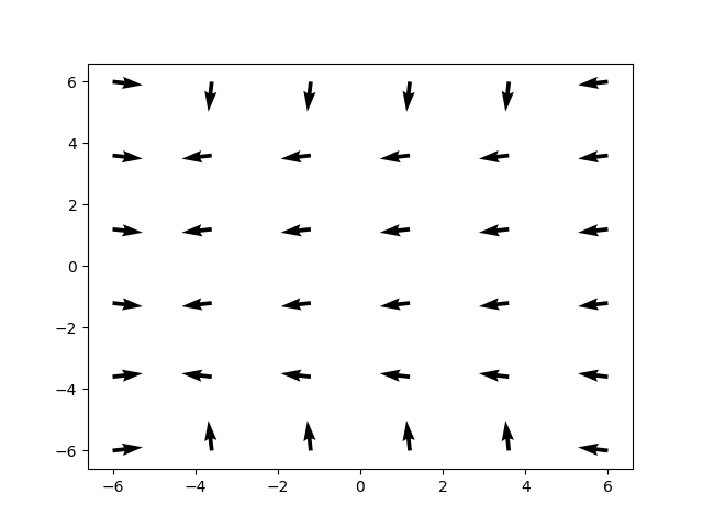
Now, this isn’t really an unmitigated success as is. I switched to an absolute value potential because GLPK_MI needs it to be linear. ECOS_BB works with a quadratic potential, but it was not doing a great job. The commercial solvers (Gurobi, CPlex, Mosek) are supposed to be a great deal better. Perhaps switching to Julia, with it’s richer ecosystem might be a good idea too. I don’t really like how the solution of the absolute value potential looks. Also, even at such a small grid size it still takes around a minute to solve. When you think about it, it is exploring a ridiculously massive space and still doing ok. There are hundreds of binary variables in this example. But there is a lot of room for tweaking and I think the approach is intriguing.
Musings:
- Can one do steepest descent style analysis for low energy statistical mechanics or quantum field theory?
- Is the trace of the mixed integer program search tree useful for perturbative analysis? It seems intuitively reasonable that it visits low lying states
- The Coulomb gas is a very obvious candidate for mixed integer programming. Let the charge variables on each grid point = integers. Then use the coulomb potential as a quadratic energy. The coulomb gas is dual to the XY model. Does this exhibit itself in the mixed integer formalism?
- Coulomb Blockade?
- Nothing special about the circle. It is not unreasonable to make piecewise linear approximations or other convex approximations of the sphere or of Lie groups (circle is U(1) ). This is already discussed in particular about SO(3) which is useful in robotic kinematics and other engineering topics.
Edit: /u/mofo69extreme writes:
By absolute value potential, I mean using $|\nabla \phi| $ as compared to a more ordinary quadratic $|\nabla \phi|^2$ .
This is where I’m getting confused. As you say later, you are actually using two fields, phi_x and phi_y. So I’m guessing your potential is the “L1 norm”
$|\nabla \phi| = |\nabla \phi_x| + |\nabla \phi_y|$ ? This is the only linear thing I can think of.
“I don’t feel that the exact specifics of the XY model actually matter all the much.” You should be careful here though. A key point in the XY model is the O(2) symmetry of the potential: you can multiply the vector (phi_x,phi_y) by a 2D rotation matrix and the Hamiltonian is unchanged. You have explicitly broken this symmetry down to Z_4 if your potential is as I have written above. In this case, the results of the famous JKKN paper and this followup by Kadanoff suggest that you’ll actually get a phase transition of the so-called “Ashkin-Teller” universality class. These are actually closely related to the Kosterlitz-Thouless transitions of the XY model; the full set of Ashkin-Teller phase transitions actually continuously link the XY transition with that of two decoupled Ising models.
You should still get an interesting phase transition in any case! Just wanted to give some background, as the physics here is extremely rich. The critical exponents you see will be different from the XY model, and you will actually get an ordered Z_4 phase at low temperatures rather than the quasi-long range order seen in the low temperature phase of the XY model. (You should be in the positive h_4 region of the bottom phase diagram of Figure 1 of the linked JKKN paper.)”
These are some interesting points and references.