Solving the Ising Model using a Mixed Integer Linear Program Solver (Gurobi)
I came across an interesting thing, that finding the minimizer of the Ising model is encodable as a mixed integer linear program.
The Ising model is a simple model of a magnet. A lattice of spins that can either be up or down. They want to align with an external magnetic field, but also with their neighbors (or anti align, depending on the sign of the interaction). At low temperatures they can spontaneously align into a permanent magnet. At high temperatures, they are randomized. It is a really great model that contains the essence of many physics topics.
Linear Programs minimize linear functions subject to linear equality and inequality constraints. It just so happens this is a very solvable problem (polynomial time).
MILP also allow you to add the constraint that variables take on integer values. This takes you into NP territory. Through fiendish tricks, you can encode very difficult problems. MILP solvers use LP solvers as subroutines, giving them clues where to search, letting them step early if the LP solver returns integer solutions, or for bounding branches of the search tree.
How this all works is very interesting (and very, very roughly explained), but barely matters practically since other people have made fiendishly impressive implementations of this that I can’t compete with. So far as I can tell, Gurobi is one of the best available implementations (Hans Mittelman has some VERY useful benchmarks here http://plato.asu.edu/bench.html), and they have a gimped trial license available (2000 variable limit. Bummer.). Shout out to CLP and CBC, the Coin-Or Open Source versions of this that still work pretty damn well.
Interesting Connection: Quantum Annealing (like the D-Wave machine) is largely based around mapping discrete optimization problems to an Ising model. We are traveling that road in the opposite direction.
So how do we encode the Ising model?
Each spin is a binary variable $ s_i \in {0,1}$
We also introduce a variable for every edge. which we will constrain to actually be the product of the spins. $ e_{ij} \in {0,1}$. This is the big trick.
We can compute the And/Multiplication (they coincide for 0/1 binary variables) of the spins using a couple linear constraints. I think this does work for the 4 cases of the two spins.
$ e_{ij} \ge s_i +s_j - 1$
$ e_{ij} \le s_j $
$ e_{ij} \le s_i $
The xor is usually what we care about for the Ising model, we want aligned vs unaligned spins to have different energy. It will have value 1 if they are aligned and 0 if they are anti-aligned. This is a linear function of the spins and the And.
$ s_i \oplus s_j = s_i + s_j - 2 e_{ij}$
Then the standard Hamiltonian is
$ H=\sum B_i s_i + \sum J_{ij} (s_i + s_j - 2 e_{ij})$
Well, modulo some constant offset. You may prefer making spins $ \pm 1$, but that leads to basically the same Hamiltonian.
The Gurobi python package actually let’s us directly ask for AND constraints, which means I don’t actually have to code much of this.
We are allowed to use spatially varying external field B and coupling parameter J. The Hamiltonian is indeed linear in the variables as promised.
After already figuring this out, I found this chapter where they basically do what I’ve done here (and more probably). There is nothing new under the sun. The spatially varying fields B and J are very natural in the field of spin glasses.
https://onlinelibrary.wiley.com/doi/10.1002/3527603794.ch4
For a while I thought this is all we could do, find the lowest energy solution, but there’s more! Gurobi is one of the few solvers that support iteration over the lowest optimal solutions, which means we can start to talk about a low energy expansion. https://www.gurobi.com/documentation/8.0/refman/poolsearchmode.html#parameter:PoolSearchMode
Here we’ve got the basic functionality. Getting 10,000 takes about a minute. This is somewhat discouraging when I can see that we haven’t even got to very interesting ones yet, just single spin and double spin excitations. But I’ve got some ideas on how to fix that. Next time baby-cakes.
(A hint: recursion with memoization leads to some brother of a cluster expansion.)
from gurobipy import *
import matplotlib.pyplot as plt
import numpy as np
# Create a new model
m = Model("mip1")
m.Params.PoolSearchMode = 2
m.Params.PoolSolutions = 10000
# Create variables
N = 10
spins = m.addVars(N,N, vtype=GRB.BINARY, name='spins')
links = m.addVars(N-1,N-1,2, vtype=GRB.BINARY, name='links')
xor = {}
B = np.ones((N,N)) #np.random.randn(N,N)
J = 1. #antialigned
H = 0.
for i in range(N-1):
for j in range(N-1):
#for d in range(2)
m.addGenConstrAnd(links[i,j,0], [spins[i,j], spins[i+1,j]], "andconstr")
m.addGenConstrAnd(links[i,j,1], [spins[i,j], spins[i,j+1]], "andconstr")
xor[i,j,0] = spins[i,j] + spins[i+1,j] - 2*links[i,j,0]
xor[i,j,1] = spins[i,j] + spins[i,j+1] - 2*links[i,j,1]
H += J*xor[i,j,0] + J*xor[i,j,1]
for i in range(N):
#m.addGenConstrAnd(links[i,N-1,0], [spins[i,N-1], spins[i+1,j]], "andconstr")
#m.addGenConstrAnd(links[N-1,j,1], [spins[i,j], spins[i,j+1]], "andconstr")
#m.addGenConstrAnd(links[i,N-1,1], [spins[i,N-1], spins[i,0]], "andconstr")
#m.addGenConstrAnd(links[N-1,j,0], [spins[i,j], spins[i,j+1]], "andconstr")
for j in range(N):
H += B[i,j]*spins[i,j]
#B[i,j] = 1.
#quicksum([2*x, 3*y+1, 4*z*z])
#LinExpr([1.]*N*N,spins)
#x = m.addVar(vtype=GRB.BINARY, name="x")
#y = m.addVar(vtype=GRB.BINARY, name="y")
# = m.addVar(vtype=GRB.BINARY, name="z")
# Set objective
m.setObjective(H, GRB.MINIMIZE)
# Add constraint: x + 2 y + 3 z <= 4
#m.addConstr(x + 2 * y + 3 * z <= 4, "c0")
# Add constraint: x + y >= 1
#m.addConstr(x + y >= 1, "c1")
m.optimize()
#for v in m.getVars():
# print(v.varName, v.x)
print('Obj:', m.objVal)
print('Solcount:', m.SolCount)
for i in range(m.SolCount):
m.Params.SolutionNumber = i #set solution numbers
print("sol val:", m.Xn)
print("sol energy:", m.PoolObjVal)
print(spins[0,0].Xn)
ising = np.zeros((N,N))
for i in range(N):
for j in range(N):
ising[i,j] = spins[i,j].Xn
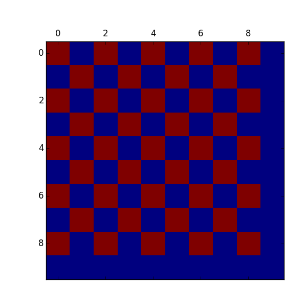
plt.matshow(ising)
plt.show()
Here’s the ground antiferromagnetic state. Cute.