PyTorch Trajectory Optimization Part 2: Work in Progress
I actually have been plotting the trajectories, which is insane that I wasn’t already doing in part 1. There was clearly funky behavior.
Alternating the Lagrange multiplier steps and the state variable steps seems to have helped with convergence. Adding a cost to the dynamical residuals seems to have helped clean them up also.
I should attempt some kind of analysis rather than making shit up. Assuming quadratic costs (and dynamics), the problem is tractable. The training procedure is basically a dynamical system.
Changed the code a bit to use more variables. Actually trying the cart pole problem now. The results seem plausible. A noisy but balanced dynamical residual around zero. And the force appears to flip it’s direction as the pole crosses the horizontal.
Polyak’s step length
http://stanford.edu/class/ee364b/lectures/subgrad_method_notes.pdf
The idea is that if you know the optimal value you’re trying to achieve, that gives you a scale of gradient to work with. Not as good as a hessian maybe, but it’s somethin’. If you use a gradient step of $ x + (f-f*)\frac{\nabla f}{|\nabla f|^2}$ it at least has the same units as x and not f/x. In some simple models of f, this might be exactly the step size you’d need. If you know you’re far away from optimal, you should be taking some big step sizes.
The Polyak step length has not been useful so far. Interesting idea though.
import torch
import matplotlib.pyplot as plt
import numpy as np
batch = 1
N = 50
T = 7.0
dt = T/N
NVars = 4

x = torch.zeros(batch,N,NVars, requires_grad=True)

#print(x)

#v = torch.zeros(batch, N, requires_grad=True)

f = torch.zeros(batch, N-1, requires_grad=True)

l = torch.zeros(batch, N-1,NVars, requires_grad=True)
#with torch.no_grad():
#	x[0,0,2] = np.pi


'''
class Vars():
	def __init__(self, N=10):
		self.data = torch.zeros(batch, N, 2)
		self.data1 = torch.zeros(batch, N-1, 3)
		self.lx = self.data1[:,:,0]
		self.lv = self.data1[:,:,1]
		self.f = self.data1[:,:,2]
		self.x = self.data[:,:,0]
		self.v = self.data[:,:,1]
'''
def calc_loss(x,f, l):
	delx = (x[:,1:,:] - x[:, :-1,:]) / dt

	xbar = (x[:,1:,:] + x[:, :-1,:]) / 2
	dxdt = torch.zeros(batch, N-1,NVars)
	THETA = 2
	THETADOT = 3
	X = 0
	V = 1
	dxdt[:,:,X] = xbar[:,:,V]
	dxdt[:,:,V] = f
	dxdt[:,:,THETA] = xbar[:,:,THETADOT]
	dxdt[:,:,THETADOT] = -torch.sin(xbar[:,:,THETA]) + torch.cos(f)


	xres = delx - dxdt

	#dyn_err = torch.sum(torch.abs(xres) + torch.abs(vres), dim=1) #torch.sum(xres**2 + vres**2, dim=1) # + Abs of same thing?

	lagrange_mult = torch.sum(l * xres, dim=1).sum(1)


	cost = 0.1*torch.sum((x[:,:,X]-1)**2, dim=1)  + .1*torch.sum( f**2, dim=1) + torch.sum( torch.abs(xres), dim=1).sum(1)*dt +  torch.sum((x[:,:,THETA]-np.pi)**2, dim=1)*0.01

	#cost = torch.sum((x-1)**2, dim=1)


	total_cost =   cost + lagrange_mult  #100 * dyn_err + reward

	return total_cost, lagrange_mult, cost, xres

#print(x.grad)
#print(v.grad)
#print(f.grad)

import torch.optim as optim
'''
# create your optimizer
optimizer = optim.SGD(net.parameters(), lr=0.01)

# in your training loop:
optimizer.zero_grad()   # zero the gradient buffers
output = net(input)
loss = criterion(output, target)
loss.backward()
optimizer.step()    # Does the update
'''

#Could interleave an ODE solve step - stinks that I have to write dyanmics twice
#Or interleave a sepearate dynamic solving
# Or could use an adaptive line search. Backtracking
# Goal is to get dyn_err quite small


'''
learning_rate = 0.001
for i in range(40):
	total_cost=calc_loss(x,v,f)
	#total_cost.zero_grad()
	total_cost.backward()
	while dyn_loss > 0.01:
		dyn_loss.backward()
		with torch.no_grad():
			learning_rate = dyn_loss / (torch.norm(x.grad[:,1:]) + (torch.norm(v.grad[:,1:])
			x[:,1:] -= learning_rate * x.grad[:,1:] # Do not change Starting conditions
			v[:,1:] -= learning_rate * v.grad[:,1:]
	reward.backward()
	with torch.no_grad():
		f -= learning_rate * f.grad
'''
learning_rate = 0.005
costs= []
for i in range(4000):
	total_cost, lagrange, cost, xres = calc_loss(x,f, l)
	costs.append(total_cost[0])
	print(total_cost)
	#print(x)
	#total_cost.zero_grad()

	total_cost.backward()
	with torch.no_grad():
		#print(f.grad)
		#print(lx.grad)
		#print(x.grad)
		#print(v.grad)
		f -= learning_rate * f.grad
		#l += learning_rate * l.grad

		#print(x.grad[:,1:])
		x[:,1:,:] -= learning_rate * x.grad[:,1:,:] # Do not change Starting conditions

	#x.grad.data.zero_()

	#f.grad.data.zero_()
	l.grad.data.zero_()
	total_cost, lagrange, cost, xres = calc_loss(x,f, l)
	costs.append(total_cost[0])
	print(total_cost)
	#print(x)
	#total_cost.zero_grad()

	total_cost.backward()
	with torch.no_grad():
		#print(f.grad)
		#print(lx.grad)
		#print(x.grad)
		#print(v.grad)
		#f -= learning_rate * f.grad
		l += learning_rate * l.grad

		#print(x.grad[:,1:])
		#x[:,1:,:] -= learning_rate * x.grad[:,1:,:] # Do not change Starting conditions

	x.grad.data.zero_()

	f.grad.data.zero_()
	#l.grad.data.zero_()


print(x)
#print(v)
print(f)

plt.plot(xres[0,:,0].detach().numpy(), label='Xres')
plt.plot(xres[0,:,1].detach().numpy(), label='Vres')
plt.plot(xres[0,:,2].detach().numpy(), label='THeres')
plt.plot(xres[0,:,3].detach().numpy(), label='Thetadotres')
plt.plot(x[0,:,0].detach().numpy(), label='X')
plt.plot(x[0,:,1].detach().numpy(), label='V')
plt.plot(x[0,:,2].detach().numpy(), label='Theta')
plt.plot(x[0,:,3].detach().numpy(), label='Thetadot')
plt.plot(f[0,:].detach().numpy(), label='F')

#plt.plot(costs)
#plt.plot(l[0,:,0].detach().numpy(), label='Lx')

plt.legend(loc='upper left')
plt.show()
Problems:
-
The step size is ad hoc.
-
Lagrange multiplier technique does not seem to work
-
Takes a lot of steps
-
diverges
-
seems to not be getting an actual solution
-
Takes a lot of iterations
On the table: Better integration scheme. Hermite collocation?
Be more careful with scaling, what are the units?
mutiplier smoothing. Temporal derivative of lagrange multiplier in cost?
alternate more complete solving steps
huber on theta position cost. Square too harsh? Punishes swing away too much?
more bullshit optimization strats as alternatives to grad descent
weight sooner more than later. Care more about earlier times since want to do model predictive control
Just solve eq of motion don’t worry about control as simpler problem
Pole up balancing
logarithm squeezing method - nope
The lambda * x model of lagrange mulitplier. Leads to oscillation
Damping term?
This learning rate is more like a discretization time step than a decay parameter. Well the product of both actually.
Heat equation model. Kind of relaxing everything into place
Made some big adjustments
Switched to using pytorch optimizers. Adam seems to work the best. Maybe 5x as fast convergence as my gradient descent. Adagrad and Adadelta aren’t quite as good. Should still try momentum. Have to reset the initial conditions after every iteration. A better way? Maybe pass x0 in to calc_loss separately?
Switched over to using the method of multipliers http://www.cs.cmu.edu/~pradeepr/convexopt/Lecture_Slides/Augmented-lagrangian.pdf
The idea is to increase the quadratic constraint cost slowly over time, while adjusting a Lagrange mutiplier term to compensate also. Seems to be working better. The scheduling of the increase is still fairly ad hoc.
import torch
import matplotlib.pyplot as plt
import numpy as np
import torch.optim
batch = 1
N = 50
T = 10.0
dt = T/N
NVars = 4
def getNewState():
x = torch.zeros(batch,N,NVars, requires_grad=True)
f = torch.zeros(batch, N-1, requires_grad=True)
l = torch.zeros(batch, N-1,NVars, requires_grad=False)
return x,f,l
def calc_loss(x,f, l, rho):
delx = (x[:,1:,:] - x[:, :-1,:]) / dt
xbar = (x[:,1:,:] + x[:, :-1,:]) / 2
dxdt = torch.zeros(batch, N-1,NVars)
THETA = 2
THETADOT = 3
X = 0
V = 1
dxdt[:,:,X] = xbar[:,:,V]
dxdt[:,:,V] = f
dxdt[:,:,THETA] = xbar[:,:,THETADOT]
dxdt[:,:,THETADOT] = -torch.sin(xbar[:,:,THETA]) + f*torch.cos(xbar[:,:,THETA])
xres = delx - dxdt
#dyn_err = torch.sum(torch.abs(xres) + torch.abs(vres), dim=1) #torch.sum(xres**2 + vres**2, dim=1) # + Abs of same thing?
lagrange_mult = torch.sum(l * xres, dim=1).sum(1)
#cost = 0
cost = 1.0*torch.sum(torch.abs(x[:,:,THETA]-np.pi), dim=1) # 0.1*torch.sum((x[:,:,X]-1)**2, dim=1) +
#cost += 2.0 * torch.sum((x[:,30:-1,THETA] - np.pi)**2,dim=1)
#cost += 7.0*torch.sum( torch.abs(xres)+ xres**2 , dim=1).sum(1)
penalty = rho*torch.sum( xres**2 , dim=1).sum(1)
# + 1*torch.sum( torch.abs(xres)+ xres**2 , dim=1).sum(1)
# 5.0*torch.sum( torch.abs(xres)+ xres**2 , dim=1).sum(1) +
cost += 0.01*torch.sum( f**2, dim=1)
#cost += torch.sum(-torch.log(f + 1) - torch.log(1 - f),dim=1)
cost += 0.1*torch.sum(-torch.log(xbar[:,:,X] + 1) - torch.log(1 - xbar[:,:,X]),dim=1)
cost += 0.1*torch.sum(-torch.log(xbar[:,:,V] + 1) - torch.log(1 - xbar[:,:,V]),dim=1)
#cost += torch.sum(-torch.log(xres + .5) - torch.log(.5 - xres),dim=1).sum(1)
# torch.sum( torch.abs(xres), dim=1).sum(1)*dt +
#cost = torch.sum((x-1)**2, dim=1)
total_cost = cost + lagrange_mult + penalty #100 * dyn_err + reward
return total_cost, lagrange_mult, cost, xres
import torch.optim as optim
learning_rate = 0.001
x, f, l = getNewState()
optimizers = [torch.optim.SGD([x,f], lr= learning_rate),
torch.optim.Adam([x,f]),
torch.optim.Adagrad([x,f])]
optimizerNames = ["SGD", "Adam", "Adagrad"]
optimizer = optimizers[1]
#optimizer = torch.optim.SGD([x,f], lr= learning_rate)
#optimizer = torch.optim.Adam([x,f])
#optimizer = torch.optim.Adagrad([x,f])
costs= []
path = []
mults = []
rho = 0.1
prev_cost = 0
for j in range(15):
prev_cost = None
for i in range(1,10000):
total_cost, lagrange, cost, xres = calc_loss(x,f, l, rho)
costs.append(total_cost[0])
if i % 5 == 0:
#pass
print(total_cost)
optimizer.zero_grad()
total_cost.backward()
optimizer.step()
with torch.no_grad():
x[0,0,2] = 0#np.pi+0.3 # Initial Conditions
x[0,0,0] = 0
x[0,0,1] = 0
x[0,0,3] = 0
#print(x.grad.norm()/N)
#print((x.grad.norm()/total_cost/N).detach().numpy() < 0.01)
#if (x.grad.norm()).detach().numpy()/N < 0.1: #Put Convergence condition here
if i > 2000:
break
if prev_cost:
if ((total_cost - prev_cost).abs()/total_cost).detach().numpy() < 0.000001:
pass #break
prev_cost = total_cost
total_cost, lagrange, cost, xres = calc_loss(x,f, l, rho)
costs.append(total_cost[0])
with torch.no_grad():
l += 2 * rho * xres
rho = rho + 0.5
print(rho)
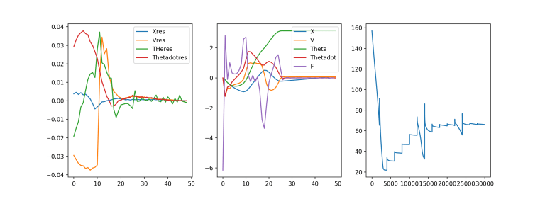
plt.subplot(131)
plt.plot(xres[0,:,0].detach().numpy(), label='Xres')
plt.plot(xres[0,:,1].detach().numpy(), label='Vres')
plt.plot(xres[0,:,2].detach().numpy(), label='THeres')
plt.plot(xres[0,:,3].detach().numpy(), label='Thetadotres')
plt.legend(loc='upper right')
#plt.figure()
plt.subplot(132)
plt.plot(x[0,:,0].detach().numpy(), label='X')
plt.plot(x[0,:,1].detach().numpy(), label='V')
plt.plot(x[0,:,2].detach().numpy(), label='Theta')
plt.plot(x[0,:,3].detach().numpy(), label='Thetadot')
plt.plot(f[0,:].detach().numpy(), label='F')
#plt.plot(cost[0,:].detach().numpy(), label='F')
plt.legend(loc='upper right')
#plt.figure()
plt.subplot(133)
plt.plot(costs)
plt.show()
The left is residuals of obeying the equations of motion, the middle is the force and trajectories themselves and the right is cost vs iteration time. Not entirely clear that a residual of 0.04 is sufficient. Integrated over time this could be an overly optimistic error of 0.2 ish I’d guess. That is on the edge of making me uncomfortable. Increase rho more? Also that force schedule seems funky and overly complex. Still, improvement from before. Feels like we’re cookin’ with gas