Gröbner Bases and Optics
Geometrical optics is a pretty interesting topic. It really is almost pure geometry/math rather than physics.
Huygens principle says that we can compute the propagation of a wave by considering the wavelets produced by each point on the wavefront separately.
In physical optics, this corresponds to the linear superposition of the waves produced at each point by a propagator function $ \int dx’ G(x,x’)$. In geometrical optics, which was Huygens original intent I think (these old school guys were VERY geometrical), this is the curious operation of taking the geometrical envelope of the little waves produced by each point.
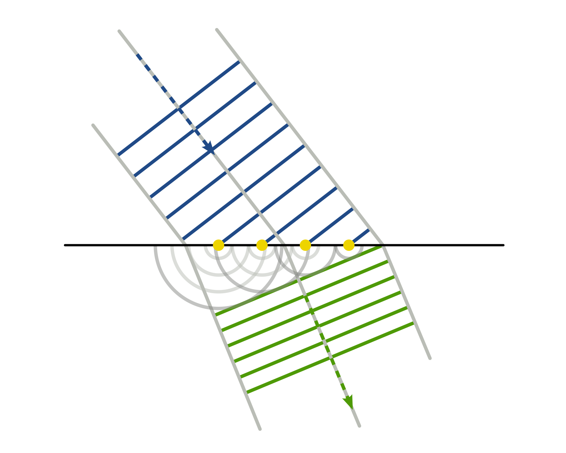 The gist of Huygens principles. Ripped from wikipedia
https://en.wikipedia.org/wiki/Envelope_(mathematics) The envelope is an operation on a family of curves. You can approximate it by a finite difference procedure. Take two subsequent curves close together in the family, find their intersection. Keep doing that and the join up all the intersections. This is roughly the approach I took in this post http://www.philipzucker.com/elm-eikonal-sol-lewitt/
 Taking the envelope of a family of lines. Ripped from wikipedia
You can describe a geometrical wavefront implicitly with an equations $ \phi(x,y) = 0$. Maybe the wavefront is a circle, or a line, or some wacky shape.
The wavelet produced by the point x,y after a time t is described implicitly by $ d(\vec{x},\vec{x’})^2 - t^2 = (x-x’)^2 + (y-y’)^2 - t^2 = 0$.
This described a family of curves, the circles produced by the different points of the original wavefront. If you take the envelope of this family you get the new wavefront at time t.
How do we do this? Grobner bases is one way if we make $ \phi$ a polynomial equation. For today’s purposes, Grobner bases are a method for solving multivariate polynomial equations. Kind of surprising that such a thing even exists. It’s actually a guaranteed terminating algorithm with horrific asymptotic complexity. Sympy has an implementation. For more on Grobner bases, the links here are useful http://www.philipzucker.com/dump-of-nonlinear-algebra-algebraic-geometry-notes-good-links-though/. Especially check out the Cox Little O’Shea books
The algorithm churns on a set of multivariate polynomials and spits out a new set that is equivalent in the sense that the new set is equal to zero if and only if the original set was. However, now (if you ask for the appropriate term ordering) the polynomials are organized in such a way that they have an increasing number of variables in them. So you solve the 1-variable equation (easy), and substitute into the 2 variable equation. Then that is a 1-variable equation, which you solve (easy) and then you substitute into the three variable equation, and so on. It’s analogous to gaussian elimination.
So check this out
from sympy import *


x1, y1, x2, y2, dx, dy = symbols('x1, y1, x2, y2, dx, dy')

def dist(x,y,d):
    return x**2 + y**2 - d**2

e1 = dist(x1,y1,2) # the original circle of radius 2
e2 = dist(x1-x2 ,y1 - y2 , 1) # the parametrized wavefront after time 1


# The two envelope conditions.
e3 = diff(e1,x1)*dx + diff(e1,y1)*1
e4 = diff(e2,x1)*dx + diff(e2,y1)*1


envelope = groebner([e1,e2,e3,e4], y1, x1, dx, dy, x2, y2, order='lex')[-1]
plot_implicit(e1, show=False)
plot_implicit(envelope, show = True)
The envelope conditions can be found by introducing two new differential variables dx, and dy. They are constrained to lie tangent to the point on the original circle by the differential equation e3, and then we require that the two subsequent members of the curve family intersect by the equation e4. Hence we get the envelope. Ask for the Grobner basis with that variable ordering gives us an implicit equations for x2, y2 with no mention of the rest if we just look at the last equation of the Grobner basis.
I set arbitrarily dy = 1 because the overall scale of them does not matter, only the direction. If you don’t do this, the final equation is scaled homogenously in dy.
This does indeed show the two new wavefronts at radius 1 and radius 3.
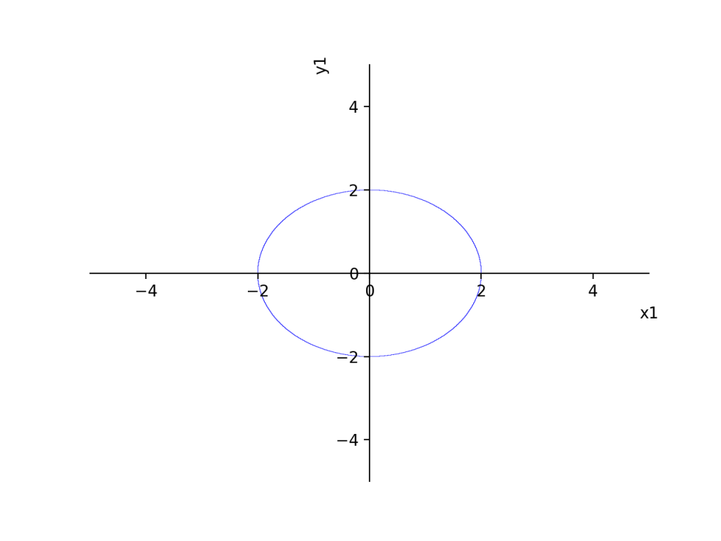 Original circle radius = 2
x12 + y12 - 4 = 0
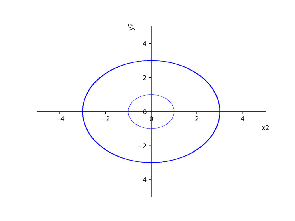 Evolved circles found via grobner basis.
(x22 + y22 - 9)*(x22 + y22 - 1) = 0
Here’s a different one of a parabola using e1 = y1 - x1 + x1**2
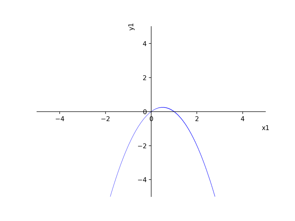 Original curve y1 - x1 + x1**2 = 0
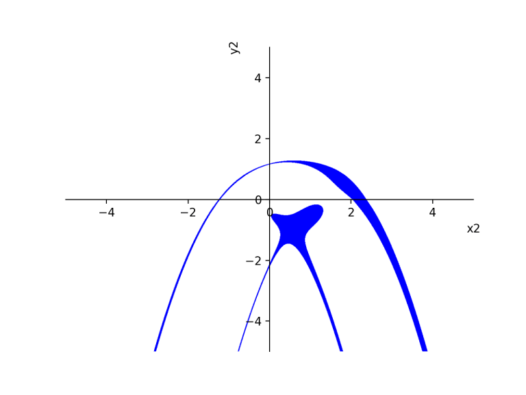 After 1 time step.
16x26 - 48*x25 + 16x24y2**2 + 32x24y2 + 4x24 - 32x2**3y22 - 64x23*y2 + 72*x23 + 32x22y2**3 + 48x22y2 - 40x22 - 32x2y23 + 16x2y22 - 16x2y2 - 4x2 + 16y24 + 32y23 - 20*y22 - 36y2 - 11 = 0
The weird lumpiness here is plot_implicit’s inability to cope, not the actually curve shape Those funky prongs are from a singularity that forms as the wavefront folds over itself.
I tried using a cubic curve x**3 and the grobner basis algorithm seems to crash my computer. :( Perhaps this is unsurprising. https://en.wikipedia.org/wiki/Elliptic_curve ?
I don’t know how to get the wavefront to go in only 1 direction? As is, it is propagating into the past and the future. Would this require inequalities? Sum of squares optimization perhaps?
Edit:
It’s been suggested on reddit that I’d have better luck using other packages, like Macaulay2, MAGMA, or Singular. Good point
Also it was suggested I use the Dixon resultant, for which there is an implementation in sympy, albeit hidden. Something to investigate
https://github.com/sympy/sympy/blob/master/sympy/polys/multivariate_resultants.py
https://nikoleta-v3.github.io/blog/2018/06/05/resultant-theory.html
Another interesting angle might be to try to go numerical with a homotopy continuation method with phcpy
http://homepages.math.uic.edu/~jan/phcpy_doc_html/welcome.html
https://www.semion.io/doc/solving-polynomial-systems-with-phcpy
or pybertini https://ofloveandhate-pybertini.readthedocs.io/en/feature-readthedocs_integration/intro.html