Fiddling around with validated ODE integration, Sum of Squares, Taylor Models.
As I have gotten more into the concerns of formal methods, I’ve become unsure that ODEs actually exist. These are concerns that did not bother me much when I defined myself as being more in the physics game. How times change. Here’s a rough cut.
A difficulty with ODE error analysis is that it is very confusing how to get the error on something you are having difficulty approximating in the first place.
If I wanted to know the error of using a finite step size dt vs a size dt/10, great. Just compute both and compare. However, no amount of this seems to bootstrap you down to the continuum. And so I thought, you’re screwed in regards to using numerics in order to get true hard facts about the true solution. You have to go to paper and pencil considerations of equations and variables and epsilons and deltas and things. It is now clearer to me that this is not true. There is a field of verified/validated numerics.
A key piece of this seems to be interval arithmetic. https://en.wikipedia.org/wiki/Interval_arithmetic An interval can be concretely represented by its left and right point. If you use rational numbers, you can represent the interval precisely. Interval arithmetic over approximates operations on intervals in such a way as to keep things easily computable. One way it does this is by ignoring dependencies between different terms. Check out Moore et al’s book for more.
What switching over to intervals does is you think about sets as the things you’re operating on rather than points. For ODEs (and other things), this shift of perspective is to no longer consider individual functions, but instead sets of functions. And not arbitrary extremely complicated sets, only those which are concretely manipulable and storable on a computer like intervals. Taylor models are a particular choice of function sets. You are manipulating an interval tube around a finite polynomial. If during integration / multiplication you get higher powers, truncate the polynomials by dumping the excess into the interval term. This keeps the complexity under wraps and closes the loop of the descriptive system.
If we have an iterative, contractive process for getting better and better solutions of a problem (like a newton method or some iterative linear algebra method), we can get definite bounds on the solution if we can demonstrate that a set maps into itself under this operation. If this is the case and we know there is a unique solution, then it must be in this set.
It is wise if at all possible to convert an ODE into integral form. $ \dot{x}= f(x,t)$ is the same as $ x(t) = x_0 + \int f(x,t)dt$.
For ODEs, the common example of such an operation is known as Picard iteration. In physical terms, this is something like the impulse approximation / born approximation. One assumes that the ODE evolves according to a known trajectory $ x_0(t)$ as a first approximation. Then one plugs in the trajectory to the equations of motion $ f(x_0,t)$ to determine the “force” it would feel and integrate up all this force. This creates a better approximation $ x_1(t)$ (probably) which you can plug back in to create an even better approximation.
If we instead do this iteration on an intervally function set / taylor model thing, and can show that the set maps into itself, we know the true solution lies in this interval. The term to search for is Taylor Models (also some links below).
I was tinkering with whether sum of squares optimization might tie in to this. I have not seen SOS used in this context, but it probably has or is worthless.
An aspect of sum of squares optimization that I thought was very cool is that it gives you a simple numerical certificate that confirms that at the infinitude of points for which you could evaluate a polynomial, it comes out positive. This is pretty cool. http://www.philipzucker.com/deriving-the-chebyshev-polynomials-using-sum-of-squares-optimization-with-sympy-and-cvxpy/
But that isn’t really what makes Sum of squares special. There are other methods by which to do this.
There are very related methods called DSOS and SDSOS https://arxiv.org/abs/1706.02586 which are approximations of the SOS method. They replace the SDP constraint at the core with a more restrictive constraint that can be expressed with LP and socp respectively. These methods lose some of the universality of the SOS method and became basis dependent on your choice of polynomials. DSOS in fact is based around the concept of a diagonally dominant matrix, which means that you should know roughly what basis your certificate should be in.
This made me realize there is an even more elementary version of DSOS that perhaps should have been obvious to me from the outset. Suppose we have a set of functions we already know are positive everywhere on a domain of interest. A useful example is the raised chebyshev polynomials. https://en.wikipedia.org/wiki/Chebyshev_polynomials The appropriate chebyshev polynomials oscillate between [-1,1] on the interval [-1,1], so if you add 1 to them they are positive over the whole interval [-1,1]. Then nonnegative linear sums of them are also positive. Bing bang boom. And that compiles down into a simple linear program (inequality constraints on the coefficients) with significantly less variables than DSOS. What we are doing is restricting ourselves to completely positive diagonal matrices again, which are of course positive semidefinite. It is less flexible, but it also has more obvious knobs to throw in domain specific knowledge. You can use a significantly over complete basis and finding this basis is where you can insert your prior knowledge.
It is not at all clear there is any benefit over interval based methods.
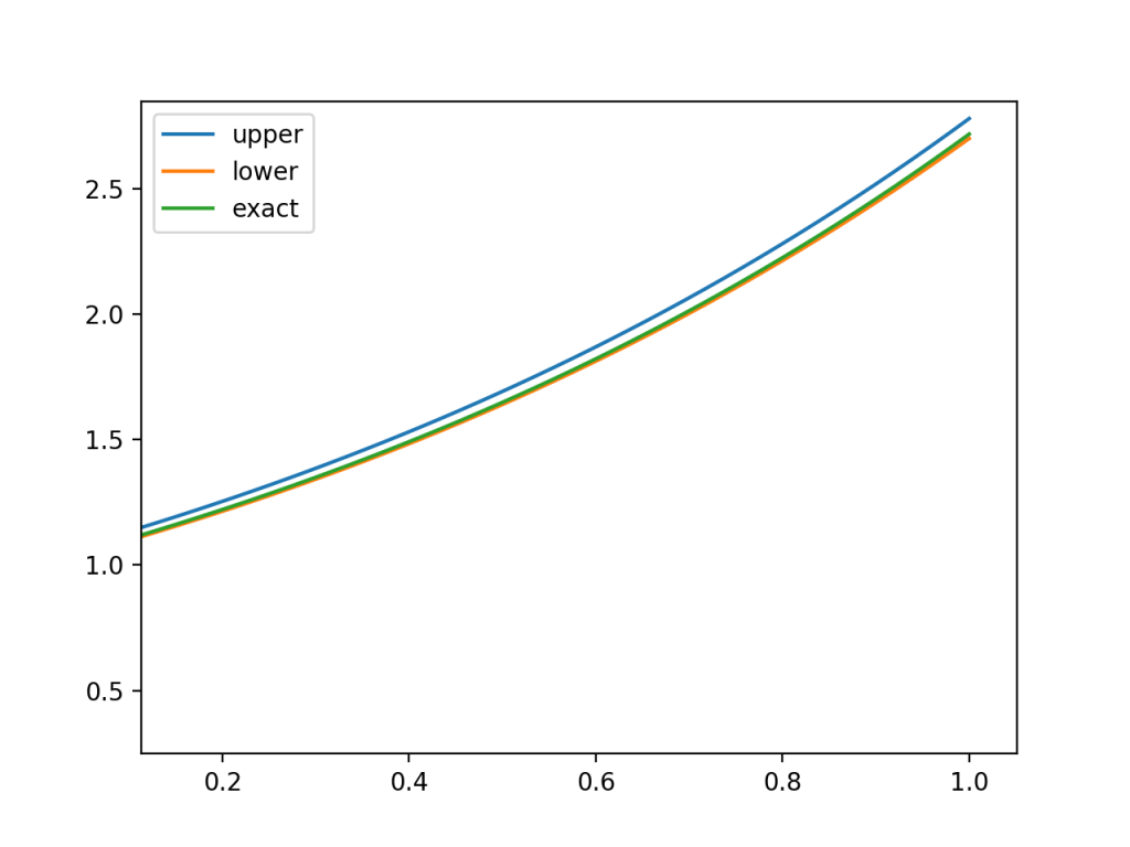
Here is a sketch I wrote for $ x’=x$ which has solution $ e^t$. I used raised chebyshev polynomials to enforce positive polynomial constraints and tossed in a little taylor model / interval arithmetic to truncate off the highest terms.
I’m using my helper functions for translating between sympy and cvxpy expressions. https://github.com/philzook58/cvxpy-helpers Sympy is great for collecting up the coefficients on terms and polynomial multiplication integration differentiation etc. I do it by basically creating sympy matrix variables corresponding to cvxpy variables which I compile to cvxpy expressions using lambdify with an explicit variable dictionary.
import cvxpy as cvx
import numpy as np
import sos
import sympy as sy
import matplotlib.pyplot as plt
#raised chebyehve
t = sy.symbols("t")

N = 5
# seems like even N becomes infeasible.
terms = [sy.chebyshevt(n,t) + 1 for n in range(N)] # raised chebyshev functions are positive on interval [-1,1]
print(terms)

'''
for i in range(1,4):
    ts = np.linspace(-1,1,100)
    #print(ts)
    #rint(sy.lambdify(t,terms[i], 'numpy')(ts))
    plt.plot( ts , sy.lambdify(t,terms[i])(ts))
plt.show()
'''

vdict = {}

l,d = sos.polyvar(terms) # lower bound on solution
vdict.update(d)

w,d = sos.polyvar(terms, nonneg=True) # width of tube. Width is always positive (nonneg)
vdict.update(d)

u = l + w # upper curve is higher than lower by width

def picard(t,f):
    return sy.integrate(f, [t,-1,t]) + np.exp(-1) # picard integration on [-1,1] interval with initial cond x(-1)=1/e

ui = picard(t,u)
li = picard(t,l)

c = []

def split(y , N): # split a polynomial into lower an upper parts.
    yp = sy.poly(y, gens=t)
    lower = sum([ c*t**p for (p,), c in  yp.terms() if p < N])
    #upper = sum([ c*x**p for (p,), c in  yp.terms() if p > N])
    upper = y - lower
    return lower,upper

terms = [sy.chebyshevt(n,t) + 1 for n in range(N+1)]

# ui <= u
lowerui, upperui = split(ui, N) # need to truncate  highest power of u using interval method
print(lowerui)
print(upperui)
du = upperui.subs(t,1)  #Is this where the even dependence of N comes from?
#c += [ du >= sos.cvxify(upperui.subs(t,1), vdict), du >= sos.cvxify(upperui.subs(t,1)]  # , upperui.subs(t,-1))
print(du)
lam1,d = sos.polyvar(terms,nonneg=True) # positive polynomial
vdict.update(d)
# This makes the iterated interval inside the original interval
c += sos.poly_eq(  lowerui + du + lam1 , u , vdict) # write polynomial inequalities in slack equality form


# l <= li
#
lam2, d = sos.polyvar(terms,nonneg=True)
vdict.update(d)
c += sos.poly_eq(  l + lam2 , li , vdict) # makes new lower bound higher than original lower bound

obj = cvx.Minimize( sos.cvxify(w.subs(t ,0.9), vdict) ) # randomly picked reasonable objective. Try minimax?
#obj = cvx.Maximize( sos.cvxify(l.subs(t ,1), vdict) )
print(c)
prob = cvx.Problem(obj, c)

res = prob.solve(verbose=True) #solver=cvx.CBC
print(res)
lower = sy.lambdify(t, sos.poly_value(l , vdict))
upper = sy.lambdify(t, sos.poly_value(u , vdict))

#plt.plot(ts, upper(ts) - np.exp(ts) ) # plot differences
#plt.plot(ts, lower(ts) - np.exp(ts)  )
ts = np.linspace(-1,1,100)
plt.plot(ts, upper(ts) , label= "upper")
plt.plot(ts, lower(ts) , label= "lower")
plt.plot(ts, np.exp(ts) , label= "exact")
#plt.plot(ts,np.exp(ts) - lower(ts) )
plt.legend()
plt.show()

'''
if I need to add in
interval rounding to get closure
is there a point to this? Is it actually simpler in any sense?

Collecting up chebyshev compoentns and chebysehv splitting would perform
lanczos economization. That'd be coo

What about a bvp

Get iterative formulation.

And what are the requirements
1. We need an iterative contractive operator
2. We need to confirm all functions that forall t, l <= f <= u
map to in between li and ui. This part might be challenging
3. Get the interval contracting and small.

x <= a
y = Lx
Lx <= La ? Yes, if positive semi definite. Otherwise we need to split it.
No. Nice try. not component wise inequality.

Secondary question: finitely confirming a differential operator is positive semi definite
forall x, xLx >= 0 ?
Similar to the above. Make regions in space.


Value function learning is contractive.
hmm.


Piecewise lyapunov functions


Being able to use an LP makes it WAY faster, WAY more stable, and opens up sweet MIPpurtunities.


'''
Seems to work, but I’ve been burned before.
man, LP solvers are so much better than SDP solvers
Random junk and links: Should I be more ashamed of dumps like this? I don’t expect you to read this.
https://github.com/JuliaIntervals/TaylorModels.jl
https://github.com/JuliaIntervals
Functional analysis by and large analyzes functions by analogy with more familiar properties of finite dimensional vector spaces. In ordinary 2d space, it is convenient to work with rectangular regions or polytopic regions.
Suppose I had a damped oscillator converging to some unknown point. If we can show that every point in a set maps within the set, we can show that the function
One model of a program is that it is some kind of kooky complicated hyper nonlinear discrete time dynamical system. And vice versa, dynamical systems are continuous time programs. The techniques for analyzing either have analogs in the other domain. Invariants of programs are essential for determining correctness properties of loops. Invariants like energy and momentum are essential for determining what physical systems can and cannot do. Lyapunov functions demonstrate that control systems are converging to the set point. Terminating metrics are showing that loops and recursion must eventually end.
If instead you use interval arithmetic for a bound on your solution rather than your best current solution, and if you can show the interval maps inside itself, then you know that the iterative process must converge inside of the interval, hence that is where the true solution lies.
A very simple bound for an integral $ \int_a^b f(x)dx$ is $ \int max_{x \in [a,b]}f(x) dx= max_{x \in [a,b]}f(x) \int dx = max_{x \in [a,b]}f(x) (b - a)$
The integral is a very nice operator. The result of the integral is a positive linear sum of the values of a function. This means it plays nice with inequalities.
Rigorously Bounding ODE solutions with Sum of Squares optimization - Intervals
Intervals - Moore book. Computational functional analaysis. Tucker book. Coqintervals. fixed point theorem. Hardware acceleration? Interval valued functions. Interval extensions.
- Banach fixed point - contraction mapping
- Brouwer fixed point
- Schauder
- Knaster Tarski
Picard iteration vs? Allowing flex on boundary conditions via an interval?
Interval book had an interesting integral form for the 2-D
sympy has cool stuff
google scholar search z3, sympy brings up interesting things
https://moorepants.github.io/eme171/resources.html
The pydy guy Moore has a lot of good shit. resonance https://www.moorepants.info/blog/introducing-resonance.html
Lyapunov functions. Piecewise affine lyapunov funcions. Are lyapunov functions kind of like a PDE? Value functions are pdes. If the system is piecewise affine we can define a grid on the same piecewise affine thingo. Compositional convexity. Could we use compositional convexity + Relu style piecewise affinity to get complicated lyapunov functions. Lyapunov functions don’t have to be continiuous, they just have to be decreasing. The Lie derivative wrt the flow is always negative, i.e gradeint of function points roughly in direction of flow. trangulate around equilibrium if you want to avoid quadratic lyapunov. For guarded system, can relax lyapunov constrain outside of guard if you tighten inside guard. Ax>= 0 is guard. Its S-procedure.
Best piecewise approximation with point choice?
http://theory.stanford.edu/~arbrad/papers/lr.ps linear ranking functions
Connection to petri nets?
https://ths.rwth-aachen.de/wp-content/uploads/sites/4/hs_lecture_notes.pdf
https://www.cs.colorado.edu/~xich8622/papers/rtss12.pdf
KoAt, LoAT. AProve. Integer transition systems. Termination analysis. Loops?
https://lfcps.org/pub/Pegasus.pdf darboux polynomials. barreir certificates. prelle-singer method. first integrals.
| method 1. arbitrary polynomial p(t). calculate p’(t). find coefficents that make p’(t) = 0 by linear algebra. Idea: near invaraints? min max | p’(t) |
Lie Algebra method
https://www.researchgate.net/publication/233653257_Solving_Differential_Equations_by_Symmetry_Groups sympy links this paper. Sympy has some lie algebra stuff in there
https://www-users.math.umn.edu/~olver/sm.html Peter Olver tutorial
http://www-users.math.umn.edu/~olver/talk.html olver talks
https://www-sop.inria.fr/members/Evelyne.Hubert/publications/PDF/Hubert_HDR.pdf
https://www.cs.cmu.edu/~aplatzer/logic/diffinv.html andre platzer. Zach says Darboux polynomials?
https://sylph.io/blog/math.html
Books: Birhoff and Rota, Guggenheimer, different Olver books, prwctical guide to invaraints https://www.amazon.com/Practical-Invariant-Monographs-Computational-Mathematics/dp/0521857015
Idea: Approximate invariants? At least this ought to make a good coordinate system to work in where the dynamics are slow. Like action-angle and adiabatic transformations. Could also perhaps bound the
Picard Iteration
I have a method that I’m not sure is ultimately sound. The idea is to start with
Error analysis most often uses an appeal to Taylor’s theorem and Taylor’s theorem is usually derived from them mean value theorem or intermediate value theorem. Maybe that’s fine. But the mean value theorem is some heavy stuff. There are computational doo dads that use these bounds + interval analysis to rigorously integrate ODEs. See https://github.com/JuliaIntervals/TaylorModels.jl
The beauty of sum of squares certificates is that they are very primitive proofs of positivity for a function on a domain of infinitely many values. If I give you a way to write an expression as a sum of square terms, it is then quite obvious that it has to be always positive. This is algebra rather than analysis.
$ y(t) = \lambda(t) \and \lambda(t) is SOS \Rightarrow \forall t. y(t) >= 0$. Sum of squares is a kind of a quantifier elimination method. The reverse direction of the above implication is the subject of the positivstullensatz, a theorem of real algebraic geometry. At the very least, we can use the SOS constraint as a relaxation of the quantified constraint.
So, I think by using sum of squares, we can turn a differential equation into a differential inequation. If we force the highest derivative to be larger than the required differential equation, we will get an overestimate of the required function.
A function that is dominated by another in derivative, will be dominated in value also. You can integrate over inequalities (I think. You have to be careful about such things. ) $ \forall t. \frac{dx}{dt} >= \frac{dx}{dt} \Rightarrow $ x(t) - x(0) >= y(t) - y(0) $
The derivative of a polynomial can be thought of as a completely formal operation, with no necessarily implied calculus meaning. It seems we can play a funny kind of shell game to avoid the bulk of calculus.
As an example, let’s take $ \frac{dx}{dt}=y$ $ y(0) = 1$ with the solution $ y = e^t$. $ e$ is a transcendental
The S-procedure is trick by which you can relax a sum of squares inequality to only need to be enforced in a domain. If you build a polynomials function that describes the domain, it that it is positive inside the domain and negative outside the domain, you can add a positive multiple of that to your SOS inequalities. Inside the domain you care about, you’ve only made them harder to satisfy, not easier. But outside the domain you have made it easier because you can have negative slack.
For the domain $ t \in [0,1]$ the polynomial $ (1 - t)t$ works as our domain polynomial.
We parametrize our solution as an explicit polynomial $ x(t) = a_0 + a_1 t + a_2 t^2 + …$. It is important to note that what follows is always linear in the $ a_i$.
$ \frac{dx}{dt} - x >= 0$ can be relaxed to $ \frac{dx}{dt} - x(t) + \lambda(t)(1-t)t >= 0$ with $ \lambda(t) is SOS$.
So with that we get a reasonable formulation of finding a polynomial upper bound solution of the differential equation
$ \min x(1) $
$ \frac{dx}{dt} - x(t) + \lambda_1(t)(1-t)t = \lambda_2(t)$
$ \lambda_{1,2}(t) is SOS$.
And here it is written out in python using my cvxpy-helpers which bridge the gap between sympy polynomials and cvxpy.
We can go backwards to figure out sufficient conditions for a bound. We want $ x_u(t_f) \gte x(t_f)$. It is sufficient that $ \forall t. x_u(t) \gte x(t)$. For this it is sufficient that $ \forall t. x_u’(t) >= x’(t) \and x_u(t_i) >= x(t_i) $. We follow this down in derivative until we get the lowest derivative in the differential equation. Then we can use the linear differential equation itself $ x^{(n)}(t) = \sum_i a_i(t) x^{(i)}(t)$. $ x_u^{(n)}(t) >= \sum max(a_i x^{(i)}_u, x^{(i)}_l)$.
$ a(t) * x(t) >= \max a(t) x_u(t), a(t) x_l(t)$. This accounts for the possibility of terms changing signs. Or you could separate the terms into regions of constant sign.
The minimization characterization of the bound is useful. For any class of functions that contains our degree-d polynomial, we can show that the minimum of the same optimization problem is less than or equal to our value.
Is the dual value useful? The lower bound on the least upper bound
Doesn’t seem like the method will work for nonlinear odes. Maybe it will if you relax the nonlinearity. Or you could use perhaps a MIDSP to make piecewise linear approximations of the nonlinearity?
It is interesting to investigtae linear programming models. It is simpler and more concrete to examine how well different step sizes approximate each other rather than worry about the differential case.
We can explicit compute a finite difference solution in the LP, which is a power that is difficult to achieve in general for differential equations.
We can instead remove the exact solution by a convservative bound.
While we can differentiate through an equality, we can’t differentiate through an inequality. Differentiation involves negation, which plays havoc with inequalities. We can however integrate through inequalities.
$ \frac{dx}{dt} >= f \and x(0) >= a \Rightarrow $ x(t) >= \int^t_0 f(x) + a$
As a generalization we can integrate $ \int p(x) $ over inequalities as long as $ p(x) \gte 0$
In particular $ \forall t. \frac{dx}{dt} >= \frac{dx}{dt} \Rightarrow $ x(t) - x(0) >= y(t) - y(0) $
We can convert a differential equation into a differential inequation. It is not entirely clear to me that there is a canonical way to do this. But it works to take the biggest.
$ \frac{dx}{dt} = A(t)x + f(t)$
Is there a tightest
We can integrate
Here let’s calculate e
https://tel.archives-ouvertes.fr/tel-00657843v2/document Thesis on ODE bounds in Isabelle
<code class="language-">myfunc x y = 3</code>
not so good. very small