A Touch of Topological Quantum Computation in Haskell Pt. I
Quantum computing exploits the massive vector spaces nature uses to describe quantum phenomenon.
The evolution of a quantum system is described by the application of matrices on a vector describing the quantum state of the system. The vector has one entry for every possible state of the system, so the number of entries can get very, very large. Every time you add a new degree of freedom to a system, the size of the total state space gets multiplied by the size of the new DOF, so you have a vector exponentially sized in the number of degrees of freedom.
Now, a couple caveats. We could have described probabilistic dynamics similarly, with a probability associated with each state. The subtle difference is that quantum amplitudes are complex numbers whereas probabilities are positive real numbers. This allows for interference. Another caveat is that when you perform a measurement, you only get a single state, so you are hamstrung by the tiny amount of information you can actually extract out of this huge vector. Nevertheless, there are a handful of situations where, to everyone’s best guess, you get a genuine quantum advantage over classical or probabilistic computation.
Topological quantum computing is based around the braiding of particles called anyons. These particles have a peculiar vector space associated with them and the braiding applies a matrix to this space. In fact, the space associated with the particles can basically only be manipulated by braiding and other states require more energy or very large scale perturbations to access. Computing using anyons has a robustness compared to a traditional quantum computing systems. It can be made extremely unlikely that unwanted states are accessed or unwanted gates applied. The physical nature of the topological quantum system has an intrinsic error correcting power. This situation is schematically similar in some ways to classical error correction on a magnetic hard disk. Suppose some cosmic ray comes down and flips a spin in your hard disk. The physics of magnets makes the spin tend to realign with it’s neighbors, so the physics supplies an intrinsic classical error correction in this case.
The typical descriptions of how the vector spaces associated with anyons work I have found rather confusing. What we’re going to do is implement these vector spaces in the functional programming language Haskell for concreteness and play around with them a bit.
Anyons
In many systems, the splitting and joining of particles obey rules. Charge has to be conserved. In chemistry, the total number of each individual atom on each side of a reaction must be the same. Or in particle accelerators, lepton number and other junk has to be conserved.
Anyonic particles have their own system of combination rules. Particle A can combine with B to make C or D. Particle B combined with C always make A. That kind of stuff. These rules are called fusion rules and there are many choices, although they are not arbitrary. They can be described by a table $ N_{ab}^{c}$ that holds counts of the ways to combine a and b into c. This table has to be consistent with some algebraic conditions, the hexagon and pentagon equations, which we’ll get to later.
We need to describe particle production trees following these rules in order to describe the anyon vector space.
Fibonacci anyons are one of the simplest anyon systems, and yet sufficiently complicated to support universal quantum computation. There are only two particles types in the Fibonacci system, the $ I$ particle and the $ \tau$ particle. The $ I$ particle is an identity particle (kind of like an electrically neutral particle). It combines with $ \tau$ to make a $ \tau$. However, two $ \tau$ particle can combine in two different ways, to make another $ \tau$ particle or to make an $ I$ particle.
So we make a datatype for the tree structure that has one constructor for each possible particle split and one constructor (TLeaf, ILeaf) for each final particle type. We can use GADTs (Generalize Algebraic Data Types) to make only good particle production history trees constructible. The type has two type parameters carried along with it, the particle at the root of the tree and the leaf-labelled tree structure, represented with nested tuples.
data Tau
data Id
data FibTree root leaves where
    TTT :: FibTree Tau l -> FibTree Tau r -> FibTree Tau (l,r)
    ITT :: FibTree Tau l -> FibTree Tau r -> FibTree Id (l,r)
    TIT :: FibTree Id l -> FibTree Tau r -> FibTree Tau (l,r)
    TTI :: FibTree Tau l -> FibTree Id r -> FibTree Tau (l,r)
    III :: FibTree Id l -> FibTree Id r -> FibTree Id (l,r)
    TLeaf :: FibTree Tau Tau
    ILeaf :: FibTree Id Id
Free Vector Spaces
We need to describe quantum superpositions of these anyon trees. We’ll consider the particles at the leaves of the tree to be the set of particles that you have at the current moment in a time. This is a classical quantity. You will not have a superposition of these leaf particles. However, there are some quantum remnants of the history of how these particles were made. The exact history can never be determined, kind of like how the exact history of a particle going through a double slit cannot be determined. However, there is still a quantum interference effect left over. When you bring particles together to combine them, depending on the quantum connections, you can have different possible resulting particles left over with different probabilities. Recombining anyons and seeing what results is a measurement of the system .
Vectors can be described in different basis sets. The bases for anyon trees are labelled by both a tree structure and what particles are at the root and leaves. Different tree associations are the analog of using some basis x vs some other rotated basis x’. The way we’ve built the type level tags in the FibTree reflects this perspective.
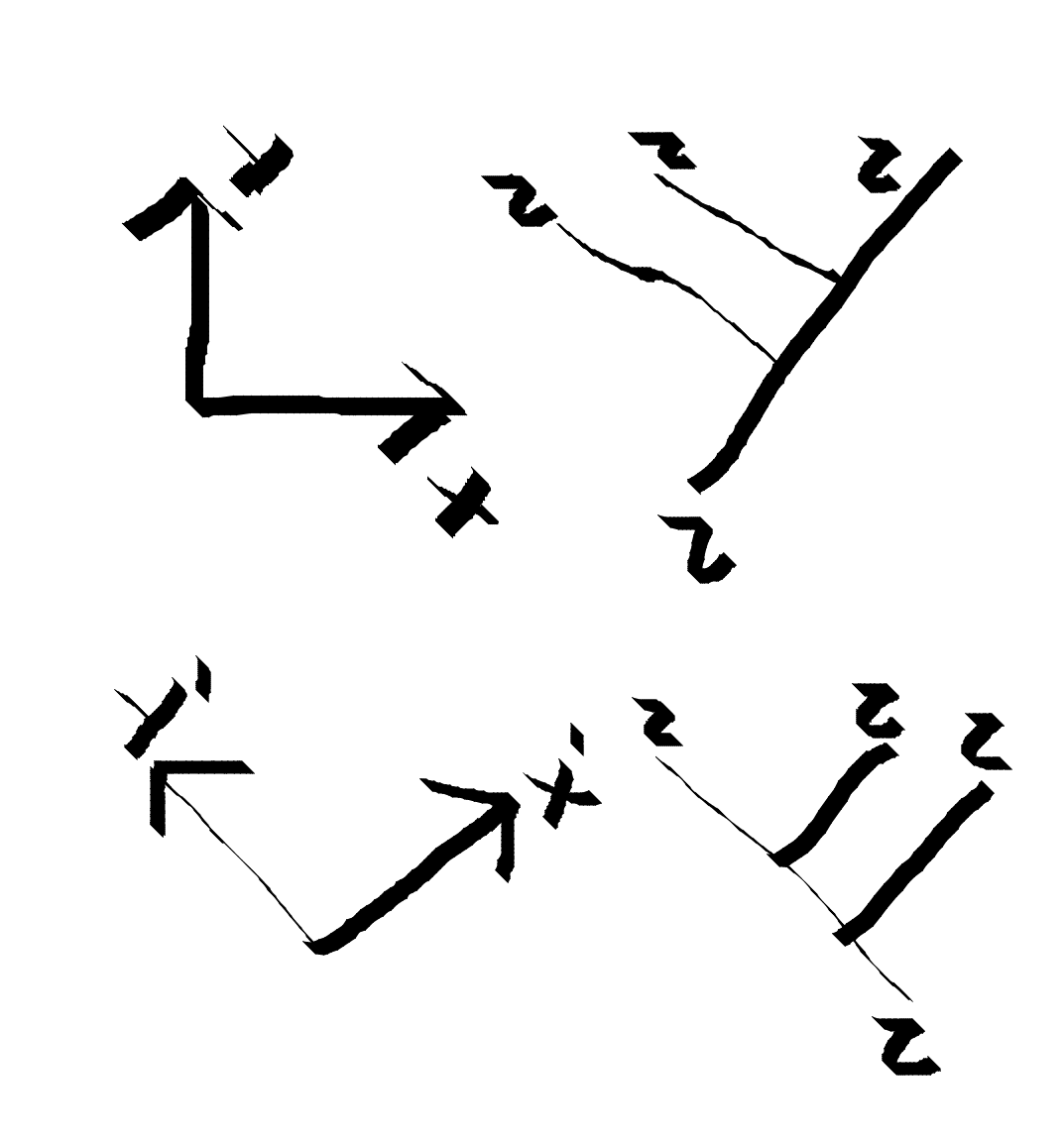
The labelling of inner edges of the tree with particles varies depending on which basis vector we’re talking about. A different inner particle is the analog of $ \hat{x}$ vs $ \hat{y}$.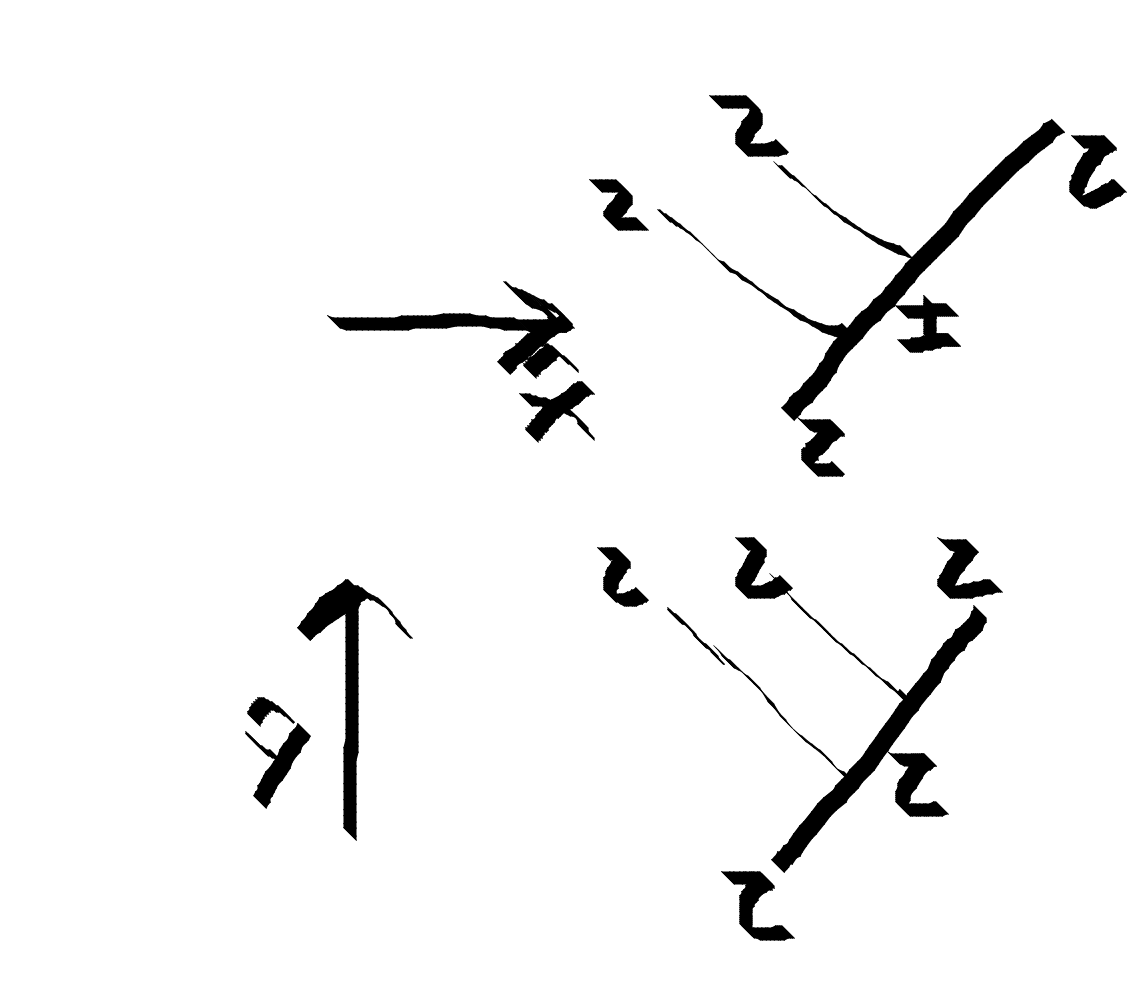
To work with these bases we need to break out of the mindset that a vector put on a computer is the same as an array. While for big iron purposes this is close to true, there are more flexible options. The array style forces you to use integers to index your space, but what if your basis does not very naturally map to integers?
A free vector space over some objects is the linear combination of those objects. This doesn’t have the make any sense. We can form the formal sum (3.7💋+2.3i👩🎨) over the emoji basis for example. Until we attach more meaning to it, all it really means is a mapping between emojis and numerical coefficients. We’re also implying by the word vector that we can add two of the combinations coefficient wise and multiply scalars onto them.
We are going to import free vectors as described by the legendary Dan Piponi as described here: http://blog.sigfpe.com/2007/03/monads-vector-spaces-and-quantum.html
What he does is implement the Free vector space pretty directly. We represent a Vector space using a list of tuples [(a,b)]. The a are basis objects and b are the coefficients attached to them.
data W b a = W { runW :: [(a,b)] } deriving (Eq,Show,Ord)
instance Semigroup (W b a) where
    (W x) <> (W y) = W (x <> y)
instance Monoid (W b a) where
    mempty = W mempty
mapW f (W l) = W $ map (\(a,b) -> (a,f b)) l
instance Functor (W b) where
    fmap f (W a) = W $ map (\(a,p) -> (f a,p)) a

instance Num b => Applicative (W b) where
    pure x = W [(x,1)]
    (W fs) <*> (W xs) = W [(f x, a * b) | (f, a) <- fs, (x, b) <- xs]


instance Num b => Monad (W b) where
    return x = W [(x,1)]
    l >>= f = W $ concatMap (\(W d,p) -> map (\(x,q)->(x,p*q)) d) (runW $ fmap f l)

a .* b = mapW (a*) b

instance (Eq a,Show a,Num b) => Num (W b a) where
        W a + W b = W $ (a ++ b)
        a - b = a + (-1) .* b
        _ * _ = error "Num is annoying"
        abs _ = error "Num is annoying"
        signum _ = error "Num is annoying"
        fromInteger a = if a==0 then W [] else error "fromInteger can only take zero argument"

collect :: (Ord a,Num b) => W b a -> W b a
collect = W . Map.toList . Map.fromListWith (+) . runW

trimZero = W . filter (\(k,v) -> not $ nearZero v) . runW
simplify = trimZero . collect
-- filter (not . nearZero . snd)

type P a = W Double a

type Q a = W (Complex Double) a
The Vector monad factors out the linear piece of a computation. Because of this factoring, the type constrains the mapping to be linear, in a similar way that monads in other contexts might guarantee no leaking of impure computations. This is pretty handy. The function you give to bind correspond to a selector columns of the matrix.
We need some way to zoom into a subtrees and then apply operations. We define the operations lmap and rmap.
lmap :: (forall a. FibTree a b -> Q (FibTree a c)) -> (FibTree e (b,d) -> Q (FibTree e (c,d)))
lmap f (ITT l r) = fmap (\l' -> ITT l' r) (f l)
lmap f (TTI l r) = fmap (\l' -> TTI l' r) (f l)
lmap f (TIT l r) = fmap (\l' -> TIT l' r) (f l)
lmap f (TTT l r) = fmap (\l' -> TTT l' r) (f l)
lmap f (III l r) = fmap (\l' -> III l' r) (f l)


rmap :: (forall a. FibTree a b -> Q (FibTree a c)) -> (FibTree e (d,b) -> Q (FibTree e (d,c)))
rmap f (ITT l r) = fmap (\r' -> ITT l r') (f r)
rmap f (TTI l r) = fmap (\r' -> TTI l r') (f r)
rmap f (TIT l r) = fmap (\r' -> TIT l r') (f r)
rmap f (TTT l r) = fmap (\r' -> TTT l r') (f r)
rmap f (III l r) = fmap (\r' -> III l r') (f r)
You reference a node by the path it takes to get there from the root. For example, (rmap . lmap . rmap) f applies f at the node that is at the right-left-right position down from the root.
Braiding
For Fibonacci anyons, the only two non trivial braidings happen when you braid two $ \tau$ particles. 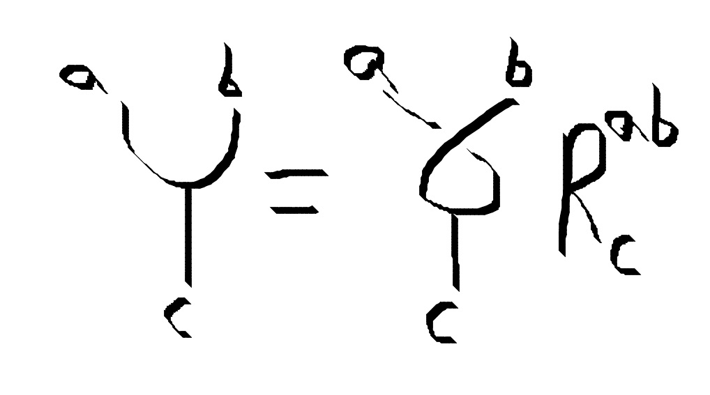
braid :: FibTree a (l,r) -> Q (FibTree a (r,l))
braid (ITT l r) = W [(ITT r l,  cis $ 4 * pi / 5)]
braid (TTT l r) = W [(TTT r l,  (cis $ - 3 * pi / 5))]
braid (TTI l r) = pure $ TIT r l
braid (TIT l r) = pure $ TTI r l
braid (III l r) = pure $ III r l

-- The inverse of braid
braid' :: FibTree a (l,r) -> Q (FibTree a (r,l))
braid' = star . braid
We only have defined how to braid two particles that were split directly from the same particle. How do we describe the braiding for the other cases? Well we need to give the linear transformation for how to change basis into other tree structures. Then we have defined braiding for particles without the same immediate parent also.
F-Moves
We can transform to a new basis. where the histories differs by association. We can braid two particles by associating the tree until they are together. An association move does not change any of the outgoing leaf positions. It can, however, change a particle in an interior position. We can apply an F-move anywhere inside the tree, not only at the final leaves.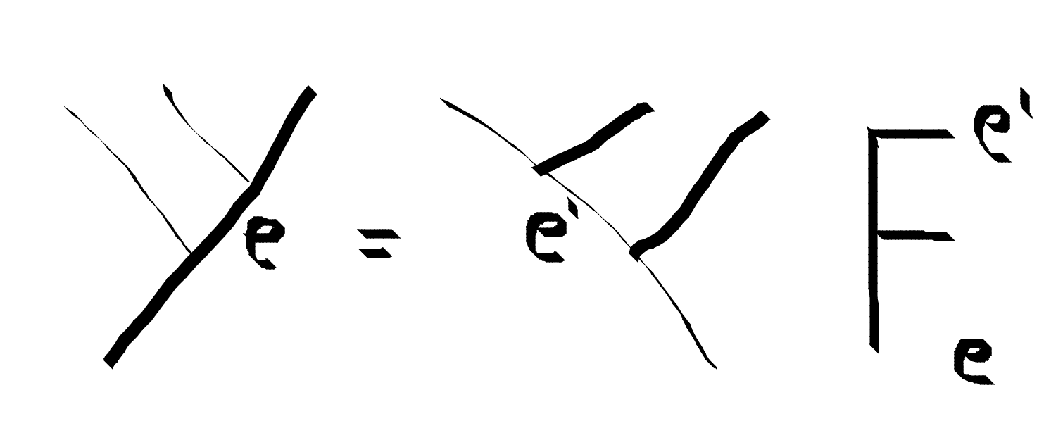
fmove :: FibTree a (c,(d,e)) -> Q (FibTree a ((c,d),e))
fmove (ITT  a  (TIT b c)) = pure $ ITT ( TTI  a b) c
fmove (ITT  a  (TTT b c)) = pure $ ITT ( TTT  a b) c
fmove (ITT  a  (TTI b c)) = pure $ III ( ITT  a b) c

fmove (TIT  a  (TTT b c)) = pure $ TTT ( TIT  a b) c
fmove (TIT  a  (TTI b c)) = pure $ TTI ( TIT  a b) c
fmove (TIT  a  (TIT b c)) = pure $ TIT ( III  a b) c

fmove (TTI  a  (III b c)) = pure $ TTI ( TTI  a b) c
fmove (TTI  a  (ITT b c)) = W [(TIT ( ITT  a b) c, tau)         , (TTT ( TTT  a b) c, sqrt tau)]

fmove (TTT  a  (TTT b c)) = W [(TIT ( ITT  a b) c, sqrt tau)  ,   (TTT ( TTT  a b) c, - tau   )]
fmove (TTT  a  (TTI b c)) = pure $ TTI ( TTT  a b) c
fmove (TTT  a  (TIT b c)) = pure $ TTT ( TTI  a b) c

fmove (III  a  (ITT b c)) = pure $ ITT ( TIT  a b) c
fmove (III  a  (III b c)) = pure $ III ( III  a b) c


fmove' :: FibTree a ((c,d),e) -> Q (FibTree a (c,(d,e)))
fmove' (ITT ( TTI  a b) c) = pure $ (ITT  a  (TIT b c))
fmove' (ITT ( TTT  a b) c) = pure $  (ITT  a  (TTT b c))
fmove' (ITT ( TIT  a b) c) = pure $  (III  a  (ITT b c))


fmove' (TTI ( TTT  a b) c) = pure $ (TTT  a  (TTI b c))
fmove' (TTI ( TTI  a b) c) = pure $ (TTI  a  (III b c))
fmove' (TTI ( TIT  a b) c) = pure $ TIT  a  (TTI b c)

fmove' (TTT ( TTI  a b) c ) = pure $ TTT  a  (TIT b c)
fmove' (TTT ( TIT  a b) c ) = pure $ TIT  a  (TTT b c)
fmove' (TTT ( TTT  a b) c) = W [(TTI  a  (ITT b c), sqrt tau)  , (TTT  a  (TTT b c),   - tau  )]


fmove' (TIT ( ITT  a b) c) = W [(TTI  a  (ITT b c), tau)         , (TTT  a  (TTT b c) , sqrt tau)]
fmove' (TIT ( III  a b) c ) = pure $ TIT  a  (TIT b c)

fmove' (III ( III  a b) c ) = pure $ III  a  (III b c)
fmove' (III ( ITT  a b) c
Fusion / Dot product
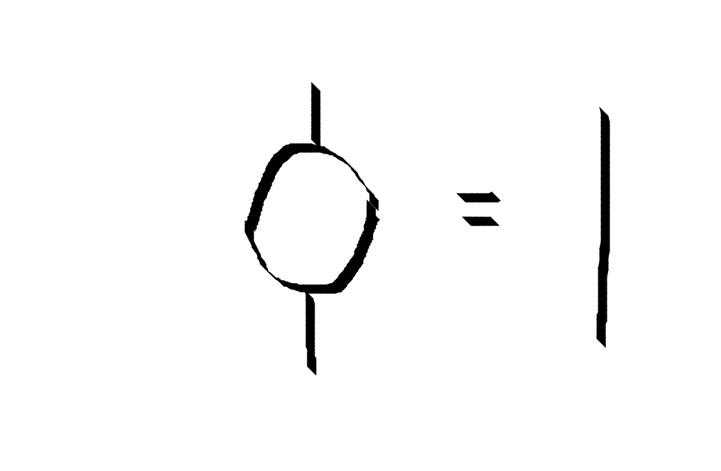
Two particles that split can only fuse back into themselves. So the definition is pretty trivial. This is like \(\hat{e}_i \cdot \hat{e}_j = \delta_{ij}\) .
dot :: FibTree a (b, c) -> FibTree a' (b, c) -> Q (FibTree a' a)
dot x@(TTI _ _) y@(TTI _ _) | x == y = pure TLeaf
                                | otherwise = mempty
dot x@(TIT _ _) y@(TIT _ _) | x == y = pure TLeaf
                                | otherwise = mempty
dot x@(TTT _ _) y@(TTT _ _) | x == y = pure TLeaf
                            | otherwise = mempty
dot x@(III _ _) y@(III _ _) | x == y = pure ILeaf
                            | otherwise = mempty
dot x@(ITT _ _) y@(ITT _ _) | x == y = pure ILeaf
                            | otherwise = mempty
dot _ _ = mempty
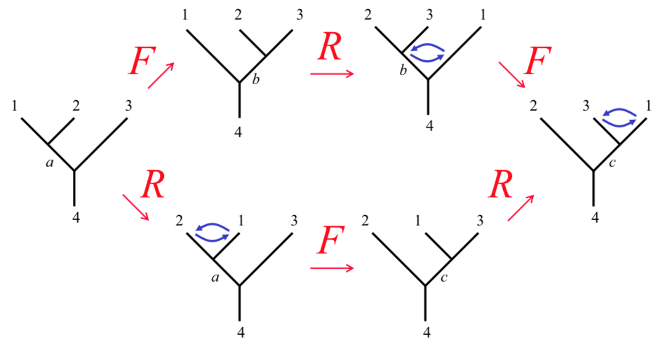
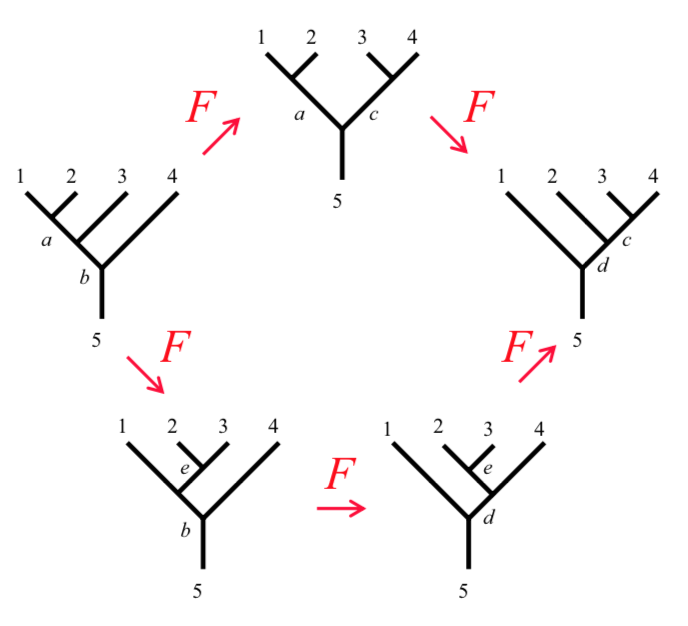
Hexagon and Pentagon equations
The F and R matrices and the fusion rules need to obey consistency conditions called the hexagon and pentagon equations. Certain simple rearrangements have alternate ways of being achieved. The alternative paths need to agree.
pentagon1 ::  FibTree a (e,(d,(c,b))) -> Q (FibTree a (((e,d),c),b))
pentagon1 v =  do
                    v1 <- fmove v
                    fmove v1

pentagon2 :: FibTree a (b,(c,(d,e))) -> Q (FibTree a (((b,c),d),e))
pentagon2 v = do
                v1 :: FibTree a (b,((c,d),e)) <- rmap fmove v
                v2 :: FibTree a ((b,(c,d)),e) <- fmove v1
                lmap fmove v2

ex1 = TTT TLeaf (TTT TLeaf (TTT TLeaf TLeaf))
-- returns empty
pentagon =  simplify $ ((pentagon1 ex1) - (pentagon2 ex1))

hexagon1 :: FibTree a (b,(c,d)) -> Q (FibTree a ((d,b),c))
hexagon1 v = do
                v1 :: FibTree a ((b,c),d) <- fmove v
                v2 :: FibTree a (d,(b,c)) <- braid v1
                fmove v2

hexagon2 :: FibTree a (b,(c,d)) -> Q (FibTree a ((d,b),c))
hexagon2 v = do
                v1 :: FibTree a (b,(d,c)) <- rmap braid v
                v2 :: FibTree a ((b,d),c) <- fmove v1
                lmap braid v2


ex2 = (TTT TLeaf (TTT TLeaf TLeaf))
--returns empty
hexagon =  simplify $ ((hexagon1 ex2) - (hexagon2 ex2))
Next Time:
With this, we have the rudiments of what we need to describe manipulation of anyon spaces. However, applying F-moves manually is rather laborious. Next time we’ll look into automating this using arcane type-level programming. You can take a peek at my trash WIP repo here
References:
John Preskill’s notes: www.theory.caltech.edu/~preskill/ph219/topological.pdf
A big ole review on topological quantum computation: https://arxiv.org/abs/0707.1889
Ady Stern on The fractional quantum hall effect and anyons: https://www.sciencedirect.com/science/article/pii/S0003491607001674
Another good anyon tutorial: https://arxiv.org/abs/0902.3275
Mathematica program that I still don’t get, but is very interesting: http://www.cs.ox.ac.uk/people/jamie.vicary/twovect/guide.pdf
Kitaev huge Paper: https://arxiv.org/abs/cond-mat/0506438
Bonderson thesis: https://thesis.library.caltech.edu/2447/2/thesis.pdf
Bernevig review: https://arxiv.org/abs/1506.05805
More food for thought:
The Rosetta Stone: http://math.ucr.edu/home/baez/rosetta.pdf
http://blog.sigfpe.com/2008/08/hopf-algebra-group-monad.html
http://haskellformaths.blogspot.com/2012/03/what-is-hopf-algebra.html
https://vimeo.com/6590617